in Modeling Cardiac Optical Mapping Measurements

) recorded when the tissue is at rest. Fluxes captured during an AP are denoted by F. The signal due only to the AP itself is $$F - F_0$$. We shall rather use the usual renormalization:


$$\begin{aligned} g^{\star } = \overline{F_0}\, \max \left( 0,\frac{F-F_0}{F_0}\right) . \end{aligned}$$

(1)
Indeed the $$\max (\ldots )$$ amounts to ignore negative, physically irrelevant, optical signals (due to noise). The multiplication by the average $$\overline{F_0}$$ of the background signal is a way to retrieve the correct amplitude of the signal. Our main goal is to reconstruct the 3D front of the AP from these 2D optical data.
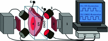
A339585_1_En_52_Fig1_HTML.gif


Fig. 1.
The optical imaging setup: (1) CCD camera, (2) emission filter, (3) LED illumination, (4) tissue sample, (5) ECG electrode, (6) bipolar stimulating electrode.


3 Model


3.1 Forward Problem


In order to write the mathematical model of these observations, we assume the following: the cameras record photon fluxes through the surfaces, the light interacts with the tissue material in the diffusive regime [2], and a Robin boundary condition can be used to model the interaction between the tissue and its environment. Hence the illumination light is described by its photon density $$\phi _0$$ that solves the diffusion equation


$$\begin{aligned} {\left\{ \begin{array}{ll} - D_0\varDelta \phi _0 + \mu _0\phi _0 = 0 \quad \text {in }\varOmega ,&{}\\ \phi _0 + d_0 \frac{\partial \phi _0}{\partial n} =0 \quad \text {on }\partial \varOmega {\setminus } \varGamma ,&{} \text {and } \phi _0 = \frac{I_0\delta _0}{D_0} \quad \text {on } \varGamma , \end{array}\right. } \end{aligned}$$

(2)
where $$\varOmega \subset {\mathbb R}^3$$ represents the slab of tissue, $$\varGamma $$ is the illuminated surface, and n is the unit normal to $$\partial \varOmega $$, outward of $$\varOmega $$. The fluorescent light is assumed to be proportional to the TMP and the illumination light (multiplicative factor $$\beta >0$$” src=”/wp-content/uploads/2016/09/A339585_1_En_52_Chapter_IEq10.gif”></SPAN>). Its photon density solves:<br />
<DIV id=Equ3 class=Equation><br />
<DIV class=EquationContent><br />
<DIV class=MediaObject><IMG alt=

(3)
In both equations, the optical parameters D, $$\mu $$, d stand respectively for diffusion coefficient, absorption coefficient and extrapolation distance. The attenuation length is the parameter $$\delta _0$$ defined by $$\delta _0 = \sqrt{\frac{D_0}{\mu _0}}$$. The intensity of the illumination, assumed uniform, is the parameter $$I_0$$. The multiplicative factor $$\beta >0$$” src=”/wp-content/uploads/2016/09/A339585_1_En_52_Chapter_IEq15.gif”></SPAN> is known for the dye used during the experiments. The dyes are assumed to be uniformly distributed in the tissue. Finally the fluxes measured through the surfaces are given by Fick’s law:<br />
<DIV id=Equ4 class=Equation><br />
<DIV class=EquationContent><br />
<DIV class=MediaObject><IMG alt=

(4)
Remark that the experimental flux $$g^{\star }$$ given by (1) does not satisfy Eq. (3), because of the renormalization. The quantity $$F-F_0$$ does. However we shall consider $$g^\star $$ as a good approximation of g, following the recommendations of the experimenters.

Since we consider a rectangular slab of tissue, we may have used structured meshes. We choose to work with unstructured meshes in order to allow more general geometries. This is necessary to study data from heart tissues. The diffusion equations are solved with P1-Lagrange finite elements method using the solver FreeFem++ [4].


3.2 Inverse Problem


The problem of retrieving the 3D spatial distribution of the TMP, denoted by $$V_m(t,{\mathbf {x}})$$ from the 2D optical signals at time $$t>0$$” src=”/wp-content/uploads/2016/09/A339585_1_En_52_Chapter_IEq20.gif”></SPAN> is under-determined. Hereafter, <SPAN id=IEq21 class=InlineEquation><IMG alt= denotes a point in $$\varOmega $$ with Cartesian coordinates (xyz). Instead of finding the complete distribution $$V_m(t,{\mathbf {x}})$$, we look for a depolarization front at each time. Specifically, we assume that a surface $${\mathcal S}(t) = \{{\mathbf {x}}\in \varOmega :\ f(t,{\mathbf {x}}) = 0\}$$ defined as the level 0 of the function f splits the domain $$\varOmega $$ into the region $$\varOmega _r = \{{\mathbf {x}}\in \varOmega :\ f(t,{\mathbf {x}}) > 0\}$$” src=”/wp-content/uploads/2016/09/A339585_1_En_52_Chapter_IEq26.gif”></SPAN> of tissue at rest, and the region <SPAN id=IEq27 class=InlineEquation><IMG alt= of excited tissue. It follows that $$V_m(t,{\mathbf {x}}) = V_p$$ if $${\mathbf {x}}\in \varOmega _p$$, and $$V_m(t,{\mathbf {x}}) = V_0$$ if $${\mathbf {x}}\in \varOmega _r$$. We consider simple depolarization fronts $${\mathcal S}$$ modeled


  • either by the sphere centered in $${\mathbf {x}}_0\in \varOmega $$ and expanding with the velocity $$c>0$$” src=”/wp-content/uploads/2016/09/A339585_1_En_52_Chapter_IEq34.gif”></SPAN> after the given time <SPAN id=IEq35 class=InlineEquation><IMG alt=, defined by the level-set function $$f(t,{\mathbf {x}}) = | {\mathbf {x}}- {\mathbf {x}}_0 | - c (t-t_0)$$,


  • or by the fixed ellipsoid centered in $${\mathbf {x}}_0\in \varOmega $$ and with radiuses $$r_x,\, r_y,\, r_z >0$$” src=”/wp-content/uploads/2016/09/A339585_1_En_52_Chapter_IEq38.gif”></SPAN>, defined by the level-set function <SPAN id=IEq39 class=InlineEquation><IMG alt=.

This level-set approach generalizes to more complex AP, once these simple cases are completely understood. In both cases, the inverse problem reduces to the identification of a small parameters set $$\mathcal {P} = ({\mathbf {x}},c,t_0) \subset {\mathbb R}^5$$ (sphere) or $$\mathcal {P}=({\mathbf {x}},r_x,r_y,r_z) \subset {\mathbb R}^6$$ (ellipsoid). In order to identify these parameters, we minimize the least squares difference $$e(\mathcal {P})$$ between the actual measurements and the measurements computed from Eqs. (2)–(4) with a TMP as above:


$$\begin{aligned} e(\mathcal {P})=\frac{1}{2}\sum _{i=1}^4 \Vert g^i_{\mathcal {P}} - g^{\star ,i} \Vert _{L^2({\mathbb S}_i)}^2, \end{aligned}$$

(5)
where the functions $$g^{\star ,i}$$ are the data. Here i refers to one of the four images ($$i \in \left\{ 1,\, 2,\, 3,\, 4\right\} $$), and the surface $${\mathbb S}_i$$ is either the epicardium or the endocardium, as detailed in Table 1. Although this is the natural way to define the cost function, the value $$I_0$$ of the illumination in Eq. (2) is unknown, while the optical parameters are. Consequently, and since Eqs. (2)–(4) are linear, the density $$\phi _0$$, or $$\phi $$, can only be computed up to a multiplicative constant. The mapping $$I_0 \mapsto g^i$$ is also linear, the measurement in-silico $$g^i$$ is consequently proportional to $$I_0$$, and we can change the cost function to account for this unknown value. A first idea is to identify the intensity $$I_0$$, and consider the following modified cost function:
Get Clinical Tree app for offline access