Lower Extremity
The anterior muscles of the thigh include the sartorius muscle (38), and the four components of the quadriceps muscle (39). The most anterior is the rectus femoris (39a), and lateral to this is the vastus lateralis (39b). The vastus intermedius (39c) and vastus medialis (39d) form the anterolateral borders of the adductor canal. This contains the superficial femoral artery and vein (119/120).
The adductor muscles comprise the superficially located gracilis muscle (38a) and the adductor longus (44a), brevis (44b), and magnus (44c) muscles. The pectineus muscle (37) is only seen in the most caudal images of the pelvis.
The posterior muscles of the thigh extend the hip joint and flex the knee joint. The group consists of the long and short heads of the biceps femoris muscle (188) and the semitendinosus (38b) and semimembranosus muscles (38c). In the proximal third of the thigh ( Fig. 159.1 ), the hypointense tendon of the biceps muscle is adjacent to the sciatic nerve (162). In the distal third of the thigh ( Fig. 159.3 ), the medial popliteal nerve (162a), which supplies the dorsal muscles, can be seen separate from the lateral popliteal nerve (162b). Note the close relationship of the profunda femoris artery and vein (119a /120a) to the femur (66) and the superficial position of the long saphenous vein (211a).


The popliteal artery (209) and vein (210), formed cranial to the joint line, are demonstrated at the level of the patella (191) in the fossa between the femoral condyles (66d) ( Fig. 160.1 ). The tibial nerve (162a) lies directly posterior to the vein, whereas the fibular (peroneal) nerve (162b) lies more laterally. The medial (202a) and lateral (202b) heads of the gastrocnemius muscle and the plantaris muscle (203a) can be seen posterior to the femoral condyles. The long saphenous vein (211a) lies medially in the subcutaneous fat covering the sartorius muscle (38), and the biceps femoris muscle (188) lies laterally.
On the section just caudal to the patella ( Fig. 160.2 ), the patellar tendon (191c) can be identified, posterior to which is the infrapatellar fat pad (2). Between the femoral condyles lie the cruciate ligaments (191b). Transverse sections such as these are frequently combined with coronal and sagittal MPRs (see also the images of a fracture on p. 167).


The muscles of the lower leg are separated into four compartments by the interosseus membrane between the tibia (189) and the fibula (190) and by the lateral and posterior intermuscular septa ( Figs. 161.1 to 161.3 ). The anterior compartment contains the tibialis anterior muscle (199), the extensor hallucis longus muscle (200a) and the digitorum longus muscle (200b) next to the anterior tibial vessels (212). The lateral compartment contains the peroneus longus (201a) and brevis (201b) muscles next to the peroneal vessels (214). In slender individuals who have no fat between the muscles, these vessels and the peroneal nerve are only poorly defined ( Fig. 161.2 ). The flexor muscles can be separated into a superficial and a deep group. The superficial group encompasses the gastrocnemius muscle with medial (202a) and lateral (202b) heads, the soleus muscle (203), and the plantaris muscle (203a). The deep group includes the tibialis posterior (205), the flexor hallucis longus (206a), and the flexor digitorum longus muscles (206b). These muscles are particularly well defined in the distal third of the lower leg ( Fig. 161.3 ). The tibil alis posterior vessels (213) and the tibial nerve (162a) pass between the two flexor groups.


The following three pages show the normal anatomy of the foot on the bone window. You will find the numbers to the legends in the back foldout.
The image series begins in a plane through the talus (192) just distal to the talocrural joint. Figure 162.1 shows the distal end of the fibula or lateral malleolus (190a) as well as the upper part of the calcaneous (193). In Figure 162.2 , the sustentaculum tali (193a) of the calcaneous is seen.


More distally, additional metatarsal bones are seen: the navicular bone (194) has begun to appear in Figure 162.2 , but its joint with the talus is better assessed in Figure 162.3 . The articular surfaces are normally smooth and the synovial space between the bones is of uniform width.


Compare these images of a normal foot with the images of fractures on pages 164 and 165.
The Achilles tendon (215), which arises from both the soleus (203) and the gastrocnemius (202) muscles, is seen posteriorly on these images.


The cuboid bone (195) is seen on the lateral margin of the foot, between the calcaneus (193) and the navicular (194). The lateral (196c), intermediate (196b), and medial (196a) cuneiform bones lie anterior to the navicular ( Fig. 163.1 ).


The transition to the metatarsal bones (197) is not always well defined, because the plane of the tarsometatarsal joints is at an oblique angle to the sections (partial volume effects ( Fig. 163.2 ). The joints can be more clearly assessed in multiplanar reconstructions that take this obliquity into account (cf. Fig. 164.1 ).
The lumbrical and quadratus plantae muscles and the short flexor muscles of the foot (208) are seen just below the arch of the metatarsal bones. These muscles are only poorly defined in CT images ( Fig. 163.3 ).


Multiplanar reconstructions are very valuable for visualizing fractures of the foot. The lateral digital radiograph in Figure 164.1a indicates the angle of the image plane, parallel to the long axis of the foot, seen in Figure 164.1b . This reconstructed image extends from the lateral (190a) and medial (189a) malleoli (at the lower edge of the image) through the talus (192) and the navicular (194) to the three cuneiform bones (196a-c). Two of the metatarsal bones (197) are included in the section. Note that the surfaces of the joints are smooth and evenly spaced. The sagittal image in Figure 164.2b was reconstructed slightly more laterally (see position in Fig. 164.2a ) so that the cuboid bone (195) is included. The short flexor muscles (208) and the plantar ligaments are seen below the arch of the foot. The Achilles tendon (215) is seen posteriorly.


Diagnosis of Fractures
Typical signs of a fracture can be seen in the original axial plane ( Fig. 164.3a ): irregularities in the cortical outline (), displaced fragments () and a fracture line () in the calcaneous. The MPR in the coronal plane (indicated in Fig. 164.3b ) shows that not only is the calcaneous () fractured, but there is a hairline fracture of the talus () involving the ankle joint ( Fig. 164.3c ).


Fractures of the foot may initially escape detection in conventional x-rays if there is no major displacement of bone fragments. If the foot remains painful, a follow-up x-ray may show the fracture because fine hairline fractures can be seen when filled with hemorrhage. As an alternative, CT would show discrete fracture lines (187), as for example of the talus (192) in Figure 165.1 .
In chronic fractures, the displaced fragment (*) has usually become rounded off ( Fig. 165.2 ). In this example, it is obvious that there were actually two fragments because a second fracture line () is seen next to the main one (187).
It is often difficult to treat comminuted fractures of the calcaneus (193), incurred for example during a fall ( Fig. 165.3 ), because there are many small displaced fragments. A stabile reconstruction of the arch of the foot may not be possible, resulting in a long period of sick leave.


The assessment of fractures of long bones is generally the domain of conventional radiology. But CT examinations are helpful for locating displaced fragments and in the preoperative planning of comminuted fractures. Infections, however, are more accurately imaged by CT than by conventional radiographs because bone destruction is more readily seen on bone windows (Fig. 166. 1c) and soft-tissue involvement (178) is documented on soft-tissue windows ( Fig. 166.1a ). This patient had septic arthritis of the left hip joint with involvement of the acetabulum (60) and femoral head (66a).
The abscess appears more clearly after contrast enhancement (cf. Figs. 166.2a and 166.2c). The increased vascularity of the wall and the fluid within the abscess (181) are well demarcated from surrounding fat (2). Adjacent muscles (38, 39, 44) are no longer individually defined because of edema (compare with the right leg). Gas (4) has been produced and is loculated in the adjacent tissues.


Related posts:


Stay updated, free articles. Join our Telegram channel

Full access? Get Clinical Tree


