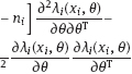
Nonlinear and generalized linear models

4Nonlinear and generalized linear models

In previous chapters, we studied some types of nonlinear regression (1.1) and considered the binary logistic regression models (1.2) and (1.3). It turns out that in these models, conditional distribution of y given ξ belongs to the so-called exponential family.

4.1Exponential family of densities

Let Y be a random variable, with distribution depending on the parameter η ∈ I. Here I = R or I is a given open interval on the real line being either finite or infinite. Let μ be a σ-finite measure on the Borel σ -algebra B(R); σ-finiteness of a measure means that the real line can be decomposed as , where An are Borel measurable sets, moreover μ(An) < ∞, for all n ≥ 1.

For example, the Lebesgue measure λ1 on B(R) is σ-finite because and λ1([−n, n ]) = 2 n < ∞, n ≥ 1.

Suppose that Y has a density function ρ(y|η) w.r.t. the measure μ. This means that for every set A ∈ B(R),

The latter integral is the Lebesgue integral (Halmos, 2013).

Definition 4.1. A density function ρ(y|η), η ∈ I , belongs to the exponential family if

Here C(·) ∈ C2(I), C″(η) > 0 for all η; ϕ > 0 is the so-called dispersion parameter; c(y, ϕ) is a Borel measurable function of two variables.

It appears that the conditional mean E(Y|η) and conditional variance D(Y|η) are expressed through the function C(·) and ϕ; moreover, E (Y|η) does not depend on ϕ.

Lemma 4.2. Assume that ρ (y|η), η ∈ I, belongs to the exponential family (4.2). Then for each η ∈ I,

Proof. Putting A = R in (4.1), we have the identity

Differentiating both sides of (4.5) with respect to η (we assume that the standard conditions allowing to apply the Leibniz rule for differentiation of an integral w.r.t. a parameter are fulfilled):

To prove formula (4.4), let us differentiate the identity having been found above:

Again, using the Leibniz rule we get

The lemma is proved.

We give several examples of exponential families.

Example 4.3 (Normal distribution). Let Y ∼ N(m, σ2), with m ∈ R and σ > 0. As the measure μ , we take the Lebesgue measure λ1 on the Borel σ-algebra B(R). Then, for Y, the density function ρ(y|m) with respect to λ1 is just the ordinary probability density function (pdf),

Transform it to the form (4.2)

Thus, the pdf satisfies Definition 4.1. Here

For the normal density function, it holds that ϕ = σ2 = DY, and this fact justifies the name of ϕ as dispersion parameter. We apply Lemma 4.2:

So, we have come to the correct results.

Example 4.4 (Poisson distribution). Suppose, Y has Poisson distribution Pois(λ), with parameter λ = eη, η ∈ R. This means that Y takes nonnegative values and

As the measure μ, we use the counting measure concentrated at integer points,

i.e., μ(A) is the number of points in the latter intersection. Then expression (4.19) specifies the density ρ(y|η) w.r.t. the measure μ

Thus, the density function satisfies Definition 4.1. Here η ∈ R , ϕ = 1, C (η) = eη, and c (y, ϕ) = c (y) = − ln(y!).

We apply Lemma 4.2:

Thus, we have obtained the correct result.

Example 4.5 (Gamma distribution). Suppose, Y has the gamma distribution Γ(α , λ), with the shape parameter α and scale parameter λ > 0. This means that Y takes positive values, and the pdf of Y is equal to

The parameter α is assumed fixed.

As the measure μ, we take the Lebesgue measure concentrated on the positive semiaxis:

Then expression (4.23) will give us the density function of Y w.r.t. the measure μ. Transform ρ(y|λ) to the exponential form

Set

Then

The density function ρ(y|λ), η < 0, belongs to the exponential family, with

Let us utilize Lemma 4.2:

Example 4.6 (Exponential distribution). Consider the distribution Γ(α , λ), with α = 1. This is exponential distribution, with the parameter λ > 0:

The density function satisfies (4.2), where

According to formulas (4.30), we have

Example 4.7 (Binary distribution, with λ = eη). Suppose that Y has the binary distribution (cf. (1.2)):

Here λ > 0. The distribution is very common in epidemiology (see discussion at the beginning of Chapter 1).

As the measure μ, we take a point measure concentrated at the points 0 and 1:

Here IA is the indicator function,

With respect to μ, the density function of Y is given as follows:

Put η = ln λ ∈ R:

For this density function, (4.2) holds with

According to Lemma 4.2, we have

The latter equality can be transformed to the classical form

Examples 4.3–4.7 demonstrate that various distributions belong to the exponential family.

4.2Regression model with exponential family of densities and measurement errors

Given the exponential family (4.2), suppose that the parameter η depends on the regressor ξ and unknown parameter β,

Here Θβ is a given parameter set, and the function (4.43) is assumed to be smooth enough. Formulas (4.2) and (4.43) define the regression of Y on ξ, and β is a regression parameter, while ϕ is a nuisance parameter.

Definition 4.8. The abovementioned regression model of Y on ξ is called generalized linear model (GLM), if the relation (4.43) has the form

Here h is a given smooth function.

Usually in the GLM, the parameter set Θβ = R2, i.e., there is no prior information about the parameters β0 and β1.

4.2.1Maximum likelihood estimator in the absence of measurement errors

Let be independent observations in the model (4.2) and (4.43). This implies that the observed couples are stochastically independent; moreover, the density function of yi w.r.t. the measure μ is given by equality (4.2), with η = ηi and ηi = η (ξi, β).

The values ξi are nonrandom in the functional case, and they are independent identically distributed random variables in the structural case.

In both cases it holds that

Then

The score function sML is equal to

If the parameter set Θβ is open, then the maximum likelihood estimator (MLE) ML is a measurable solution to the equation

Under mild conditions, the estimator is strongly consistent:

It is also asymptotically normal:

Here Φ is a positive definite matrix of size p×p. In the structural case, Φ is the so-called Fisher information matrix,

Using (4.47), we evaluate the matrix

The first term is zero, because

Therefore,

Since C″ > 0, the matrix Φ is positive definite, if the components of vector are linearly independent in the space L2(Ω, P) of random variables. Usually, the latter holds true.

Indeed, in the GLM (4.44),

If h′ (t) ≠ 0, t ∈ R, and the random variable ξ is not constant, then the components of vector are linearly independent in L2(Ω, P ), and thus, the information matrix (4.54) is positive definite.

Remark 4.9. In the functional case (when ξi are nonrandom), the matrix Φ from relation (4.50) is found as follows:

Come back to the structural case. Having estimated β one can, if necessary, estimate the dispersion parameter ϕ. From formulas (4.3) and (4.4), we obtain

Therefore, the unbiased estimating equation for ϕ takes the form

This equation should be considered in tandem with equation (4.48). Then the estimator of the parameter ϕ is equal to

Due to the convergence (4.49) and the SLLM, one can show that a.s.,

i.e., is strongly consistent. This fact holds in the functional case as well.

4.2.2Quasi-likelihood estimator in the presence of measurement errors

Consider the regression model (4.2) and (4.43). Let a surrogate variable x be observed instead of ξ

the random vector (y, ξ)T and δ be stochastically independent, and also the pdf ρ(δ) of the classical error be known. It is assumed that Eδ = 0. By the observations , , we estimate the model parameters.

Note that in Section 1.4, we presented estimation methods in the model (1.1) and (1.5), which is a particular case of the model (4.2), (4.43), and (4.62). This is due to the fact that the normal pdf belongs to the exponential family (see Example 4.3). Now, we apply these estimation methods to the general model.

The naive estimator naive is defined by the estimating function (4.47), in which the observed values of the surrogate variable x are substituted instead of the unobserved values of the latent variable ξ. Thus, naive is a measurable solution to the equation

The estimator is not consistent even in the linear measurement error model (Theorem 2.3). The reason for the inconsistency is bias of the estimating function sML(y, x; β) (yet the unbiasedness of an estimating function is a prerequisite for the consistency of an estimator, see Appendix A1). Indeed,

Here η = η (x, β) and ; we have exploited the indifferentiability of error δ (Section 1.4.3) in the calculation

From equality (4.64), it is obvious that in general case, EβSML(y, x; β) ≠ 0, so the estimating function sML(y, x; β) is biased.

The naive estimator can be used under relatively small measurement error variances , then the asymptotic deviation of the estimate naive from the true value will be small.

To construct the quasi-likelihood (QL) estimator, we write down the conditional mean and conditional variance of y given x. To do this, assume the following:

(i) The errors δi are identically distributed, with distribution , where is positive and known.