of Polivinylalcohol Cryogel Material Model in FEM Simulations on Deformation of LV Phantom

Fig. 1.

Schematics of the left ventricle phantom, where * marks the part simulating the LV and ** the fixing collar.

Proposed geometry resulted in 52 ml volume which is in agreement with physiological end-systole volume of left ventricle [5]. A tubular collar was added for mounting physical phantoms in the laboratory setup. Stiffer inclusions were created as cylinders with main axes normal to the surface of the phantom, crossing it 40 mm from the base. This study concerns a homogenous phantom and a phantom with a transmural inclusion with diameter of 20 mm.

2.3 FEM Modeling

Numerical model of the phantom geometry, created using the Autodesk Inventor 2012 software (Autodesk Inc., USA) was exported in CAD format to the Finite Element simulation software – Abaqus 6.13-3 (Simulia, USA). The phantom was meshed into linear hexaheadral elements (type C3D8H). The collar was divided into 7020 elements via 3 mm seeding, the phantom into 7176 elements (seed 3 mm) and the inclusion into 2080 elements (seed 1, 5 mm).

The PVA cryogel was modeled as an elastic and as a hyperelastic material based on strain-stress relation derived from experiments. Elastic material was defined as isotropic with Poisson’s ratio 0, 45 and with Youngs modulus obtained by fitting a linear function to the experimental data using linear regression. The hyperelastic material was defined as isotropic, with 3-rd order Yeoh strain energy potential definition, with Poisson’s ratio 0, 45 and with stress-strain relation taken directly from measurements [4].

In the simulations the phantom was fixed by immobilizing both internal and external surfaces of the mounting collar. Deformation was forced by applying pressure load to the inner surface of the elliptical part of the phantom. The pressure linearly increased in 20 steps reaching 12 kPa. Except to the standard global coordinate system, a cylindrical system was defined, with radial direction corresponding to the radial direction of the phantom and longitudinal direction aligned with the phantoms’ main axis.

As a result of finite element analysis values of logarithmic strains at all nodes were returned by the FEM software. A set of nodes defining a line-of-interest crossing the inclusion in the direction of phantom long axis was defined (Fig. 2). Three normal strain components for points of this set were exported from Abaqus for further processing in Matlab 2012b (Mathworks, USA). The logarithmic strains ε_log have been transformed to the engineering strains ε_eng [6]:

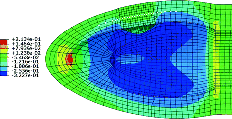
Fig. 2.

Radial strain color map for the hyperelastic phantom with the inclusion (stiffness × 3). Nodes defining the line-of-interest are marked white.

$\varepsilon_{eng} = exp\left( {\varepsilon_{log} } \right) - 1$

(1)

3 Results

3.1 PVA Characteristics

Measured relation between strain and stress is shown in the Fig. 3 in blue color. “Stiffer” variations of the PVA are a result of scaling of this relation by 1.5, 2 and 3. A linear function fitted to the data resulted in Young’s modulus values presented in the legend box in the Fig. 3.

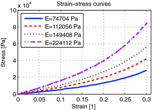
Fig. 3.

Stress-strain curves. Solid line – from measurements, dashed, dotted and with markers as a result of scaling by factors of 1.5, 2 and 3 respectively (Color figure online).

3.2 Modeling Results

Series of 3D logarithmic strain maps were obtained in Abaqus software (Fig. 2). Plots of strains as a function of distance from the first node, counting from the base, were created to assess the strain profile across the inclusion. For more compact presentation of results a measure of strain contrast C has been proposed:

$C = \frac{{\left| {\overline{{\varepsilon_{ph} }} - \overline{{\varepsilon_{inc} }} } \right|}}{{\left| {\overline{{\varepsilon_{ph} }} } \right|}} \cdot 100$

(2)

Where $\overline{{\varepsilon_{ph} }}$ is the mean strain in the phantom material along the line-of-interest and $\overline{{\varepsilon_{inc} }}$ is the mean strain in the inclusion.

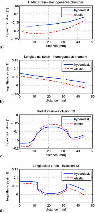
Fig. 4.

Radial and longitudinal strain plots along the line-of-interest for homogenous phantom (a) and (b) and for the phantom with an inclusion 3x stiffer than surrounding material (c) and (d) (Color figure online).

Radial, circumferential and longitudinal strains were examined. Figure 4 shows selected strain profiles – radial and longitudinal for the homogenous phantom (a and b) and for the phantom with an inclusion of highest stiffness (c and d). Each plot shows a profile for elastic (dashed red) and hyperelastic (blue) material model. Relative root mean squared differences (RRMSD) between strain profiles for the two material models are presented in the Table 1.

Strain contrasts calculated using the proposed formula (2) for both material models and all relative stiffness values proposed in Sect. 2.1 are given in Table 2. Contrasts obtained for the hyperelastic model are also presented as plots in Fig. 5, that shows additionally how the contrasts increase with increase of relative stiffness of the inclusion.

Table 1.

Root mean squared differences between strain profiles for elastic and hyperelastic material model.

Only gold members can continue reading. Log In or Register to continue