Oncology Drug Development

Edward Ashton

Philip F. Murphy

James O’Connor

Developments over the past two decades in the targeting of therapeutics, not just to particular diseases but also to specific mutations and genetic markers, combined with new methods for rapidly identifying larger numbers of target molecules, have placed an increasing strain on both the pharmaceutical industry and academic research funding agencies. From 1993 to 2003, the pharmaceutical industry and the National Institutes of Health spending both more than doubled, while the number of new molecules submitted to the Food and Drug Administration for review dropped by roughly half over that same period. Clearly, these trends are not sustainable in the long term. It is vitally important, therefore, to identify their root causes and determine which of them might be correctable.

One key cost driver in the drug development process is the rate of late-stage failure. It has been estimated that the average cost of bringing a new compound to market approval in the United States at $808 million. Other estimates have ranged as high as $1.7 billion. The bulk of these funds, clearly, are expended in the later stages of development. The Tufts study estimated that improved early screening could reduce the total capitalized cost per approved drug by $242 million, primarily by increasing the overall success rate for compounds entering early clinical trials from the current 21.5% to 30%.

A major reason for the prevalence of late-stage failure is that in many development programs demonstration of treatment effect in a human population is not attempted until phase 2, with the result that large amounts of capital can be sunk into a compound without any serious evidence that it might be successful. The decision to limit phase 1 studies to questions of safety has been driven by practical considerations. Most clinical endpoints—survival, functional scores, pain—are dependent on many factors other than drug effects, most prominently including subjectivity on the part of both patients and clinicians. These endpoints are therefore very noisy in a statistical sense and require large patient populations to achieve statistically significant results.

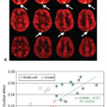
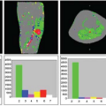
There are numerous cancer therapeutics either approved or currently in development that are either antiangiogenic or vascular disruptive agents.¹^,²^,³ The ability to accurately and precisely estimate parameters related to blood flow and vascular permeability is critical to the early evaluation of these compounds, as this gives the most direct window into their targeted biologic effects. As an example, consider the recent phase 1 trial of the vascular disruptive agent denibulin (MN-029) in patients with advanced solid tumors.⁴ This was a standard dose-escalation trial including 34 patients spread across 10 dose levels, with eight patients at the maximum tolerated dose. This sample size is not remotely adequate to demonstrate either the clinically significant or dose-dependent treatment effect using traditional clinical trial endpoints such as overall survival, progression-free survival, or overall response rate. Nevertheless, 24 of these patients were assessed for changes in blood flow and vascular permeability within target tumors 6 to 8 hours after the administration of the first dose, using dynamic contrast-enhanced magnetic resonance imaging (DCE-MRI). A plot comparing reduction in tumor vascular function postdose to denibulin exposure (Fig. 69.1) shows not only that a significant treatment effect is present in these patients, but also that the magnitude of the treatment effect is highly correlated to drug exposure.

It is important to understand what a plot of this sort does and does not demonstrate. The presumptive mechanism of action for this compound is inhibition of microtubule assembly, resulting in disruption of the cytoskeleton of tumor vascular endothelial cells. If effective, this disruption should manifest as a reduction in blood flow and vascular permeability within solid tumors. It is hypothesized that this reduction will lead to periods of transitory ischemia and tumor cell death. In this study, imaging using DCE-MRI was able to demonstrate a statistically significant and dose-dependent reduction in blood flow and vascular permeability within target tumors.

Note that although this validates the expected mechanism of action for this compound, this is not equivalent to demonstrating that patients received clinical benefit. Successful demonstration of efficacy using functional imaging techniques such as DCE-MRI is best thought of as a necessary but in no way sufficient condition for the eventual approval of the compound. Unless and until a very strong link can be established between changes in vascular parameters and clinical outcomes, these results cannot be used to demonstrate clinical efficacy. But if a compound’s primary mechanism of action is antivascular or antiangiogenic activity and no such activity is seen in early trials, it is a reasonably safe bet that even in larger trials, no clinical benefit will be forthcoming. Functional
imaging techniques such as DCE-MRI are therefore useful in the drug development process primarily as screening tools, allowing ineffective compounds to be abandoned early in the development process when relatively little time and money have been expended.

FIGURE 69.1. Scatter plot comparing area under the curve AUC_0–24h (ng·h/mL) for drug exposure based on blood draws for MN-029 to percentage change in K^trans (transfer constant) from baseline to 6 to 8 hours postdose for each of the 24 evaluable patients.

Although there are a small number of examples of clinical trials in oncology using perfusion assessment techniques such as dynamic susceptibility contrast (DSC) MRI, arterial spin labeling (ASL), and DCE computed tomography (CT), DCE-MRI is currently by far the most commonly used method in this arena. The reasons for this are fairly straightforward. As stated, the most common use of functional imaging in drug development is as a screening tool in phase 1 and early phase 2 clinical trials. In oncology, in order to maximize potential recruitment, these trials are most often either “all-comer” trials, in a broad disease area such as solid tumors, or focused on one of the common cancer types (such as breast, colorectal, lymphoma). Although DCE-MRI is generally usable anywhere in the body, DSC-MRI and ASL are somewhat more limited, DSC-MRI by susceptibility artifacts and the requirement that contrast agents remain intravascular, and ASL by the need to identify and label a clear feeder artery to the target tumor. DCE-CT is not limited in its utility, but it does carry a very heavy radiation burden, which can make institutional review board approval of a DCE-CT study problematic. Because of this, the bulk of the following discussion will be focused on DCE-MRI. Nevertheless, it should be understood that the principles outlined here for the most part apply equally well to these other techniques. Important differences between DCE-MRI, DSC-MRI, and DCE-CT are outlined below.

DCE-CT is in general a very similar technique, both in aims and capabilities, to DCE-MRI. The same models can be used with either method, and the iodinated contrast agents used in DCE-CT are similar in their pharmacokinetics (the way in which the compounds distribute themselves within the body) to the gadolinium-based agents used with DCE-MRI. There are, however, advantages and disadvantages to each technique that must be understood to select the proper approach for a particular drug development program.

The primary advantages of DCE-CT are speed and simplicity. A multislice CT scanner can easily acquire a volume in less than 1 second with high resolution (<1 mm) and good signal-to-noise ratios, whereas MRI systems are significantly more limited in terms of both spatial and temporal resolution. Additionally, the relationship between signal intensity changes seen in a CT scan and concentration of contrast agent in tissue is linear and is not dependent on the precontrast signal.

In addition to its advantages, of course, DCE-CT has several significant drawbacks. The most obvious of these is the substantial radiation dose administered to the patient during the course of the scan, which may involve the acquisition of 30 to 60 scans of the same volume over a period of less than 60 seconds. The actual dose in millisieverts will vary depending on the region being imaged. Nevertheless, as a point of reference, a single chest-abdomen-pelvis CT scan delivers roughly 10 mSv. As a point of comparison, the total allowable annual dose for a nuclear worker in the United States is 50 mSv, and standards in many countries are as low as 20 mSv.

For DSC-MRI, acquisition time is a severely limiting factor when working with T₁-weighted images. However, gadolinium-based contrast agents also affect both T₂– and T₂^*-weighted images. T₂^*-weighted images in particular are an attractive option because of their potential for high acquisition speed relative to T₁-weighted images. Acquisition times of 0.2 seconds per slice for T₂^*-weighted images are easily achievable using echo-planar imaging techniques. As should be expected, however, there are a number of differences in the way contrast concentration changes affect T₂^*-weighted images that must be understood if this technique is to be used for perfusion assessment.

First and most obviously, the presence of intravascular contrast in T₂^*-weighted images causes a reduction in observed signal intensity (darkening) rather than increased
signal intensity (brightening) as in T₁-weighted images. More significantly, the induced change in signal relative to background noise levels at a given contrast concentration is substantially lower in T₂^*-weighted images than it is in T₁-weighted images. As a result, the contrast agent dose administered for a DSC-MRI acquisition is higher than that for a DCE-MRI acquisition. Typical values are 0.1 mmol/kg for T₁-weighted images versus 0.2 to 0.3 mmol/kg for T₂^*-weighted images.

The most intractable issue associated with DSC-MRI, however, is that echo-planar imaging sequences are very strongly affected by magnetic susceptibility artifacts. They are therefore ill suited for use in regions of the body containing significant amounts of air space, such as the chest or abdomen. They are also ill suited for use with extravascular contrast. This is a severe drawback insofar as gadolinium-labeled contrast agents generally are able to cross from the capillary bed into the extravascular-extracellular space even in normal tissues, and even more so in tumors, whose capillaries typically have poorly formed and highly permeable endothelia. Gadolinium-labeled contrast agents are generally not, however, able to cross an intact blood–brain barrier, with the result that they are essentially intravascular agents within the brain.

As a result of these limitations, despite the apparent attractiveness of this technique from a speed standpoint, DSC-MRI is used almost exclusively for assessing perfusion within the brain at this time.

Measurement Variability

In order to use these tools with confidence, of course, it is vital to understand the reliability of the measurements derived from DCE-MRI and other related techniques. Reliability in this context is most often assessed in terms of the scan–rescan coefficient of variability (CoV), defined as the standard deviation divided by the mean for the parameter of interest over repeated measurements in the absence of biologic change. This measure provides a means to determine whether the changes observed in a single patient (e.g., the reduction seen in K^trans the volume transfer constant from arterial space to extracellular extravascular space in a particular tumor after antivascular therapy) are statistically significant, with a change of more than twice the CoV indicating a statistically significant treatment effect. Note that this is entirely separate from the concept of a clinically significant treatment effect; it is entirely possible to have a statistically significant response to therapy, which has no effect whatsoever on disease progression. CoV for a given population (and therefore the threshold for statistically significant change in that population) can be estimated using a relatively small number of patients. Determining a clinically significant level of change requires a much larger and more detailed dataset.

The most common method used to assess scan–rescan CoV in a clinical trial is to make use of a dual baseline protocol, in which patients are scanned twice within a narrow time window prior to the initiation of therapy. A typical protocol might leave a minimum of 2 days between scans to allow contrast washout, and a maximum of 7 to 10 days to minimize the amount of true biologic change between scans. A population CoV estimate for each parameter can then be obtained through the following process:

For each pair of measurements (baseline 1, baseline 2), calculate both mean and standard deviation.
For each pair of measurements, produce an adjusted standard deviation by multiplying the standard deviation by 1.25331 for an unbiased estimation. This step is intended to compensate for the bias resulting from estimation of the standard deviation using n = 2.
For each pair of measurements, produce a local CoV by dividing the adjusted standard deviation by the mean.
Produce a population CoV by averaging the local CoV across all pairs.

A limited number of publications have examined the expected scan–rescan CoV for perfusion parameters estimated using DCE-MRI and other related techniques.⁵^,⁶^,⁷^,⁸^,⁹^,¹⁰ Estimates of CoV for various perfusion parameters in these studies range from a low value of approximately 7% to a high of approximately 22%. This is a broad range. Nevertheless, upon closer reading, several patterns become apparent, which make it possible to narrow down estimates of CoV for a particular study.

FIGURE 69.2. Two-compartment model for the analysis of dynamic image data.

First, variability is heavily dependent on the choice of analysis model. Most perfusion analyses are based on a two compartment linear system model, as illustrated in Figure 69.2. The input to the system is provided by the time–concentration curve for contrast agent in the arterial plasma compartment, generally referred to as the arterial input function (AIF). The output is provided by the time–concentration curve for contrast agent in the extracellular-extravascular space. The properties of the vascular bed are represented by the transfer function h(t), which relates these two curves. Models such as the generalized kinetic model,¹¹ which assume a form for this function and require only the estimation of a small number of parameters, will generally provide better reproducibility.
Models such as the distributed parameter model,¹² which require the direct estimation of the transfer function via deconvolution, will generally be more susceptible to both noise and artifact and therefore provide relatively poorer reproducibility.

The reader will note that this discussion focuses heavily on precision (reproducibility) while skirting the question of absolute accuracy. There are two reasons for this. First, accuracy is a much more difficult question to address in the context of flow and permeability measurements using DCE-MRI. Because the processes being measured are dynamic, standard image or sacrifice animal experiments might be used to assess the accuracy of, for example, tumor volume measurements, which are not applicable to these techniques. Also, it is not clear that absolute accuracy is particularly important in this context, because what is typically assessed in cancer patients using DCE-MRI is change in parameter values between pre- and posttreatment imaging sessions. So, even if a particular technique produces results that are consistently biased high by 20% relative to another method, both will produce the same change estimate.

Second, variability is heavily dependent on the accuracy of the estimation of the AIF for a particular scan. A number of approaches to AIF estimation have been proposed and tested. One common approach is to avoid this problem by making use of a general concentration–time curve such as that used by Weinmann et al.¹³ However, using a theoretical AIF ignores differences in injection rate and cardiac output, which can vary from subject to subject and even with a single subject over time.⁵ These differences can greatly reduce measurement reproducibility. Galbraith et al.⁶ have reported thresholds for statistically significant change over time in K^trans in a single tumor using this method of 45% negative and 83% positive.

A second option is for an analyst to draw a manual region of interest within an artery, and use the mean enhancement curve within that region of interest as the subject-specific AIF, as described by Vonken et al.¹⁴ This approach is complicated by the fact that the MR signal in arteries is frequently corrupted by inflow artifacts, with the result that regions of interest at different points in the same artery or in other nearby vessels can provide grossly different enhancement curves. It should be noted that these artifacts are sequence dependent and are worse for two-dimensional methods than for central regions of three-dimensional methods. Even at 6-second resolution there is a big difference between the AIF and venous output function. Some have attempted to address these issues by using signal from a vein rather than an artery to minimize inflow and partial volume artifacts. Nevertheless, the uptake curve observed in the venous system is significantly different from that in the arterial system, and as a result this approach is likely to introduce significant bias into measured parameters.

Several groups have described methods for the automated or semiautomated identification of a patient-specific arterial input function using either information from large arteries present in the scan⁷^,¹⁵^,¹⁶ or a model-based derived AIF using information taken from normal reference tissues such as muscle.¹⁷ Scan–rescan variability data on these various methods is not widely available in the literature. Nevertheless, available evidence indicates that systems using automated, patient-specific AIF derivation generally show lower variability, as would be expected.⁵^,⁶^,⁷^,⁸^,⁹

There are a number of other potential sources of variability in DCE-MRI acquisition and analysis and methods to address, some of which are still lacking scientific consensus. Two prominent examples are correction of B1 inhomogeneities in the acquired DCE-MRI data and correction of raw signal differences to absolute millimolar gadolinium concentration. In both these cases, it can be argued that the correction can introduce more noise than it removes. At this time a definitive study to determine if this is indeed the case is still lacking.

Functional Imaging Biomarkers as Clinical Trial Endpoints

Endpoints for Regulatory Approval versus Endpoints for Drug Development Decision Making

Regulators require substantial evidence of safety and clinical benefit (i.e., efficacy) of a drug for marketing authorization to be granted, with data typically provided from large phase 3 studies. In oncology clinical trials, the gold standard indicator of benefit remains overall survival, but accelerated approval regulations allow the use of a surrogate endpoint, defined as an endpoint expected to predict true clinical benefit.¹⁸^,¹⁹ Confirmation of clinical benefit must then be subsequently demonstrated. The term surrogate endpoint is formally used in this context of providing evidence to regulators. To use a surrogate endpoint for this purpose, substantial validation activities are required to ensure robust statistical linkage between a shorter-term endpoint and a clinical endpoint.²⁰ Optimization of endpoints for drug registration will continue to evolve as the compromise is established between availability of important new medicines versus the strength of the data regulators need to judge effectiveness.²¹

Endpoints within the earlier phases of clinical testing have greater scope for transforming the drug development process by providing robust decision-making tools to ensure the best drug candidate is selected, the drug mechanism is understood, the right disease is targeted, the right dosing strategy is followed, and, where relevant, an optimum combination therapy is pursued. This approach will
lead to a more informed early clinical trial process, derisking drug development by ensuring that only high-quality drug candidates are progressed to more costly phases of development. If a flow of better candidates are pursued in the right patients, regulatory submission will provide ever-stronger evidence of treatment effect, and this will ultimately reduce the debate over surrogate endpoints that demonstrate small treatment effects. Therefore, a significant focus is required to develop and apply biomarkers able to provide early phase clinical trials with increasingly informative endpoints. In order to apply such endpoints for internal decision making, how well developed should a biomarker be, and how should such methods be incorporated into the clinical trial framework?

Imaging Biomarker Development

Imaging biomarker development remains an important endeavor in the advancement of clinical trial design and methodology.²² For clinical trial application, key areas of biomarker development include: (a) gaining evidence that the method can inform a relevant aspect of the pharmacology, (b) defining where the approach can optimally support drug development, for example, titrating with dose or providing some metric of efficacy, (c) enhancing robustness of measurement, particularly when broader multicenter use of a method is required, and (d) simplification so that a biomarker can be applied cost-effectively with an ever-increasing industry focus on clinical trial efficiency.

Qualification has been accepted as a term for the process by which evidence is generated linking the biomarker with a known biologic process or clinical endpoint. Although the terms validation and qualification are sometimes used interchangeably, there are important differences. Wagner²³ and Wagner et al.²⁴ outline these differences and propose a framework for qualification. For functional imaging biomarkers, qualification is the most appropriate process for determining when sufficient evidence to use the imaging biomarker has been generated.

Formalizing Imaging Biomarkers into the Clinical Trial Framework

To consider how imaging biomarkers can be optimally incorporated into clinical trials, it is important to review the definition of endpoints within the clinical trial framework. The Geek Box provides generally agreed-upon definitions from multiple sources. This categorization of endpoints into primary, secondary, and exploratory weights the roles of these endpoints for evaluating the hypothesis that the drug is effective and safe. The primary endpoint should be a well-characterized measurement (of efficacy or safety) that is easily interpreted and robustly implemented. The primary endpoint is the most important decision-making endpoint for a given trial. Typically, multiple secondary endpoints are then added to consider different aspects of drug efficacy or safety that can support the primary endpoint. Exploratory endpoints can be added and would tend to be based on methods that are not well understood in the given setting and where interpretation is potentially ambiguous. However, a clinical drug trial remains an important vehicle for developing an understanding around new methodologies that could be subsequently used in other trials. Therefore, value can likely be gained from a careful implementation of exploratory endpoints across clinical development programs, although developing new biomarkers in the context of an unknown drug effect might not always be optimum.²⁵

Geek Box

Terminology around biomarkers and endpoints for clinical trials. See Atkinson et al.,¹⁹ Wagner,²³ and Wagner et al.²⁴ for expanded definitions.

Definitions

Biomarker: A characteristic that is objectively measured and evaluated as an indicator of normal biological processes, pathogenic processes, or pharmacologic responses to a therapeutic intervention.²

Surrogate endpoint: A biomarker that is intended to substitute for a clinical endpoint. A surrogate endpoint is expected to predict clinical benefit (or harm or lack of benefit or harm) based on epidemiologic, therapeutic, pathophysiologic, or other scientific evidence.²²

Clinical endpoint: A variable that reflects how a patient feels, functions, or survives.

Biomarker validation: The process of linking a surrogate endpoint to a clinical endpoint.

Biomarker qualification: The evidentiary process of linking a biomarker with biological processes and clinical endpoints.²²

Primary endpoint: A variable able to provide the most relevant and convincing evidence directly related to the primary objective of the trial.

Secondary endpoint: A variable providing additional and supportive characterization of the treatment effect.

Exploratory endpoint: A variable that is not sufficiently characterized to be able to impact clinical trial decision making but may provide ancillary information and implementation will support development of the endpoint itself.

As an example, consider a phase 1 clinical trial of a drug that is expected to have antiangiogenic or antivascular properties. The primary endpoint in such a trial is likely to be safety and tolerability of the drug, expressed
in terms of significant adverse events observed at differing dose levels and ultimately in a maximum tolerated dose. Secondary endpoints might include change in vascular function posttherapy as measured using DCE-MRI and clinical response rate. Exploratory endpoints might include less well-established markers, such as a change in cellular density assessed using diffusion-weighted MRI.

Initially, functional imaging methodologies were predominantly incorporated into clinical trials as exploratory endpoints because the performance of the method was often characterized as poorly as the drug under development. Furthermore, technical complexity led to many examples where insufficient functional imaging data were collected (e.g., equipment failure). Nevertheless, with improvement in methodology (general robustness and standardization of acquisition and analysis) and an improved understanding of functional imaging response across different therapeutics, methods such as DCE-MRI have become accepted as important secondary endpoints. This implies that these methods are sufficiently well characterized to be able to inform drug development. DCE-MRI will tend not to provide primary study endpoints because (a) when used within a phase 1 study, safety and pharmacokinetic characterization of the drug remain the primary study objectives and (b) in phase 2 studies, weight is given to broader efficacy measurements (e.g., response rate) with the expectation that such challenging thresholds of defining response will give greater predictability for evaluating subsequent phase 3 success.

In summary, how a functional imaging biomarker is optimally incorporated into a clinical trial is dependent upon a number of key questions: Is the endpoint sufficiently well characterized that it will contribute to a key decision regarding the drug? If added as a decision-making endpoint, how would the results be used? If the endpoint is not well understood for a given trial, it might be appropriate to add it as an exploratory endpoint, where it might not impact the trial outcome but will support method development for future studies.

Clinical Feasibility of Trial Design

Once it is judged that functional imaging is to be integrated into a clinical trial, two broad areas need to be considered: How will the endpoint be incorporated into the clinical protocol? How practically will the method be implemented to ensure the highest quality data are delivered?

In designing the imaging component within the trial, the clinical context and expectations around what the method will provide are paramount. If the imaging is not practical for the investigational center or the examination burden is too great for the subjects, data will simply not be collected. Therefore, a balance must be reached between the ideal experimental design and pragmatism.

Before implementation is considered, it is vital to consider what the imaging endpoint is expected to achieve: (a) simply define some pharmacological evidence, (b) studying through a range of drug doses to establish pharmacokinetic and pharmacodynamic (the way in which the drug affects the body) relationships, or (c) understanding timing of the drug response, perhaps to optimize the use of an additional therapy.

The factors discussed in the following sections should be considered when designing the clinical trial.

Number of Scan Time Points

As mentioned previously, more than one baseline scan might provide important repeatability metrics to support response interpretation and in addition could inform on-site performance.²⁶ However, three scanning time points can be challenging for the following reasons: (a) acceptability for the subject; (b) scheduling complexity for the participating center; (c) trial costs for the sponsor; (d) multiple doses of contrast agent in some clinical settings can be problematic. Moreover, if three scanning time points are deemed feasible, the value of two baseline measurements versus follow up at two time points should be carefully considered. The issue of burden on the patient is paramount and the MRI component must be considered in the context of all other clinical trial procedures (e.g., biopsy, blood collections, CT scanning). The majority of studies published have selected two or three measurements, and most use a single baseline measurement, with estimates of measurement CoV taken from the scientific literature for similar imaging and analysis techniques.

Scan Timing

Selection of the posttreatment time point is a critical decision in the design of the trial. A later imaging time point (e.g., after multiple weeks) will reflect chronic drug dosing, providing a summary of the exposure of the drug over a long duration. After such time, multiple factors associated with the drug can impact measurement (e.g., development of central necrosis). It is known from multiple studies that some drugs can result in measurable vascular changes within hours of drug dosing that then persist (e.g., tyrosine kinase inhibitors). These early time points may successfully describe the antiangiogenic effect without contribution from other nonvascular effects and therefore should offer a more “clean” pharmacodynamic measurement. It is also known that vascular disrupting agents result in a rapid onset of vascular change, which could then return to near baseline state, therefore, early measurement is likely to be important. Nevertheless, given how little information is known about the likely onset time, it is possible that such an early measurement could miss measurement of response in some drugs and with some dosing strategies. Also, early after a drug dose,
pharmacokinetic variability may significantly add to interpatient differences in response. If two follow-up time points are feasible, it might be prudent to select one early time point that is less sensitive to early pharmacokinetic effects (such as 2 to 7 days) and a second time point after chronic exposure (e.g., 3 to 4 weeks) perhaps at a time that can be scheduled on the same day as other measurements. Later time points could also be used to study the impact of withdrawal or a scheduled drug holiday on the vasculature²⁷ or to study what drives tumor resistance and ultimately progression. Posttreatment measurement timing could be directed by preclinical studies, perhaps comparing response timing with a clinically characterized drug.

Number of Subjects Required

The size of phase 1 trials is typically governed by the phase 1 design, where the intention is to determine the maximum tolerated dose by increasing the dose level from one subject cohort to the next.²⁸ Each cohort typically comprises three to six subjects.²⁹ Given the primary objectives of typical phase 1 trials, statistical powering of the functional imaging component is generally not considered. Nevertheless, the objective is usually to maximize the amount of data available from the trial by scanning as many subjects as practically possible and minimizing methodologic failure. In particular, in studies in which dose is increased across small cohorts of subjects (e.g., three), it is important to maximize successful scanning across all those subjects at a given dose level. This is especially important when considering response heterogeneity across subjects and the fact that at lower doses the drug might only impart a slight vascular effect. So the aim of functional imaging in phase 1 studies should be to maximize the amount of high-quality imaging data collected.

Phase 2 trials are intended to evaluate therapeutic efficacy toward a specific indication, and endpoints, such as response rate, generally require a large cohort to define statistical significance, although there are continual efforts to optimize the efficiency by the design and optimal use of endpoints.³⁰^,³¹^,³² Within a phase 2 trial, there is generally more flexibility (compared with a phase 1 trial) for considering the sample size of a secondary endpoint, and functional imaging can often be implemented as a substudy. The definition of substudy could be based on a subset of subjects (e.g., with disease readily measureable by functional imaging) or only conducted at selected investigational centers, perhaps one with specific imaging expertise.

Type of Disease and Lesion Selection

Tumor Type

Given that different tumors can result in differences in vascular response, the ideal study would be to examine the functional imaging response in a single histological tumor type as studied at phase 2. Phase 1 studies, however, are typically designed to enable recruitment of subjects with advanced, refractory disease resulting in a heterogeneous cohort. Also, with an increasing number of drugs available that target the vasculature, it is possible that prior therapy with an agent different from the one being investigated will alter the baseline vascular characteristics. Either way, such patients should be excluded from participating in the functional imaging component or the timing because previous therapy should be considered. If such prior therapy is permitted in a given trial, it should be considered as a confound when interpreting vascular response.

Lesion Size and Location

In advanced disease there are often multiple lesions that could be selected for evaluation by functional imaging. Functional imaging techniques such as DCE-MRI are often unable to image the entire body in one session. As a result, a more limited set of target lesions is generally selected for assessment and is assumed to be representative of the patient’s overall disease burden. Selecting the optimal lesions to study is important and usually based on size and location. For example, with most methods, it is generally preferable to study a lesion that is at least 2 cm in diameter. In terms of lesion location, the challenge of lesion motion should be considered. With an adequate approach to motion compensation and consideration during analysis, even lung lesion measurements can be successful.³³ Because it would tend to add complexity and increase the likelihood of poor quality data, it would be prudent to study alternative, representative lesions when possible.

Number of Investigation Centers

Participating center selection is an important consideration when planning study feasibility. Most investigational centers are selected for their ability to recruit patients and their experience of conducting clinical trials to a high quality. Unfortunately, center selection does not always take into account expertise and experience with functional imaging methods. Often better data are obtained cost-effectively by focusing efforts on high-quality data acquisition at a small number of expert centers rather than trying to enable all participating centers to contribute data that might be of poor quality or at least add variability. It is important to note that the cost of implementing processes for standardized scanning and centralized analysis can become a significant percentage of the clinical trial costs. A decision around the number of investigational centers should consider scientific objectives (subjects required), practical constraints (cost, timelines), and the quality of data required.

Only gold members can continue reading. Log In or Register to continue