Other MRI Approaches to Perfusion Imaging (ASL, DSC, DCE)
2.1 The Perfusion Parameters: The Microvascular Network and Physiological Principles
Perfusion characterizes the microvascular network. The “micro” scale refers here to the size of the capillary diameter: about 6 μm. From an in vivo imaging point of view, this scale is far below the voxel size (about 1000 μm). Therefore, each voxel of a perfusion map contains hundreds or even thousands of microvessels. The perfusion value associated with that voxel is generally a mean value across these numerous microvessels. Obtaining quantitative values is not always easy and not always useful, from a clinical point of view. Often, relative index values are derived. The available perfusion estimates primarily depend on the choice of acquisition method. In most cases, several parameter maps may be derived from one acquisition. A list of examples is shown in Table 2.1.
Table 2.1 Main perfusion-related parameters that can be monitored with MRI perfusion techniques

2.2 Perfusion Tracers
To estimate perfusion parameters, imaging techniques generally rely on tracers. A perfusion tracer is a molecule introduced in the blood stream in small quantities and that does not perturb perfusion. For practical reasons, all clinical tracers are plasmatic. Indeed, labeling erythrocytes is a complex procedure not adapted to a routine clinical setting.
We will first introduce how tracers may be used to quantify perfusion parameters, from a biophysical point of view, without considering the imaging part. Then, we will consider how imaging tracers, also called contrast agents (CAs), impact the magnetic resonance imaging (MRI) signal and how MRI can be turned into perfusion MRI.
Injection mode: To avoid any increase in arterial pressure, tracers are injected into the venous system. Then, the left heart distributes the tracer into the arterial system at a physiological pressure. In addition, tracers are generally flushed with saline to ensure that the tracer reaches a large vein (i.e., the vena cava) as a bolus (<5 s).
At the organ level: From a biophysical point of view, tracers are either diffusible or nondiffusible. In other words, during the imaging sequence (or imaging session), a tracer either extravasates or remains intravascular. This depends on the organ of interest. The same tracer may be diffusible for a particular organ and nondiffusible for another (e.g., a gadolinium chelate is diffusible in the skin but not in the brain). The behavior of the tracer depends on its size (the hydrodynamic diameter), its charge, its lipophilicity, etc. The extravasation may be passive (e.g., driven by the concentration gradient between intra- and extravascular spaces) or active (e.g., active transport by vesicles) or a combination of both. In the healthy brain, capillaries are impermeable to MRICAs in almost every region [1], unless the blood–brain barrier is altered. From a biophysical point of view, a diffusible tracer is generally modeled as a tracer that passively crosses the vessel wall at a rate characteristic of the vessel wall permeability and then freely diffuses into the extravascular space.
In blood: The temporal evolution of the tracer concentration in the feeding arteries of the organ of interest is called the arterial input function (AIF). Evaluating the AIF is the most challenging part in perfusion studies. Following the intravenous injection, the left heart distributes the tracer into the arterial system and every organ sees a “first pass” of the tracer. The evolution of the tracer concentration in the draining veins of the organ of interest is called the venous output function (VOF). The interorgan difference in tracer circulation time (approximately 15 to 40 s) [2] and in blood volume is such that a second pass can be visible in some organs (such as the brain) before the tracer concentration becomes homogeneous across the entire vascular system.
Finally, the tracer concentration in blood decays. The exact mechanisms of tracer excretion depend on the tracer and are outside the scope of this chapter. Pharmaceutical companies may provide an estimate of the plasmatic half-lives for tracers for various species, including humans [3].
2.3 Biophysical Modeling of Nondiffusible Tracers
Considering an organ and a nondiffusible CA for that organ, there are two main strategies to obtain perfusion-related parameters: a dynamic approach and a steady-state approach.
2.3.1 Dynamic Approach
This approach, used in dynamic susceptibility contrast (DSC) MRI or in perfusion CT, was proposed by Hering as the ‘‘indicator dilution method’’ in 1824 [4]. Considering the tracer concentration over time in arterial blood, AIF(t), and in a particular voxel, C voxel(t), and assuming a bolus injection, no extravasation of tracer, and no tracer recirculation, the blood volume fraction (BVf), may be computed as:
(2.1)
Eq. 2.1 shows that the area under the concentration time curve of each voxel is proportional to voxel BVf. For flow, F, the following relationship holds:
(2.2)
where R(t) is the residue function. Following the arrival of an infinitely short dose of tracer, the residue function is the remaining fraction of that dose of tracer in the voxel at time t. This function decays from 1 (at t = 0, all the tracer is in the voxel) to 0 (at long t values, all the tracer has left the voxel). Deconvolving C voxel(t) by AIF(t) yields the function F∙R(t). The deconvolution is very sensitive to noise and has to be made insensitive to the tracer arrival delay [5]. In theory, the value of this function at t = 0 provides an estimate of F since R(0) = 1. In practice, there is a delay between the AIF and the tracer concentration time course in the voxel, which may be characterized by the time of the maximum of R(t), called T max [6].
A last important principle is the central volume theorem, established by Meier and Zierler [7]. Under the assumptions described above, blood volume, blood flow (F), and mean transit time (MTT) are related:
(2.3)
Assuming that the microvascular network inside the voxel has one input and one output, MTT is the mean time taken by the CA to travel along the possible microvascular pathways between the input and the output.
2.3.2 Steady-State Approach
In this approach, measurements are performed before and after the injection of a CA, once the CA concentration in blood may be considered homogeneous and stable for the acquisition duration. The ratio between the blood and the voxel CA concentrations is the voxel BVf, assuming the CA remains purely intravascular. The required stability in the intravascular CA concentration limits the scope of usable CAs.
The steady-state and dynamic approaches may be coupled: The data obtained at beginning and at the end of the dynamic acquisition may be used to perform a steady-state analysis of BVf. As the steady- state analysis does not depend on an AIF, the BVf estimate can be used to refine the dynamic analysis, such as in the book end approach [8].
2.4 Biophysical Modeling of Diffusible Tracers
We now consider an organ and a diffusible CA—an exogenous tracer such as a gadolinium chelate or simply intravascular water. Three physiological situations may be considered [9]:
- The flow-limited situation, in which the permeability is high compared to the flow. The flow is thus the limiting factor to the arrival of the tracer into the tissue. This case is the one considered if water is used as a tracer, such as in arterial spin labeling (ASL).
- The permeability-limited situation, where the flow maintains an almost constant concentration of the tracer across the vascular system in the voxel and a small fraction of the tracer extravasates.
- The mixed situation, where both flow and permeability limit the arrival of the tracer to the tissue. This case is the one generally considered in dynamic contrast–enhanced (DCE) MRI.
From a formal point of view, these situations may be described by the extraction fraction, E, that is, the fraction of tracer within blood that enters the tissue compartment:
(2.4)
where P is the permeability of the vessel wall (in cm∙s–1) and S is the surface of the vessel wall (in cm²). The permeability-surface product PS is thus a flux of tracer through the vessel wall, like F is the flux of blood through the vessels. As tracers are generally plasmatic, there is a hematocrit factor between the blood and the plasmatic concentrations of the CA.
To measure perfusion parameters, there is again a dynamic approach and a steady-state approach.
The dynamic approach, used in DCE MRI, relies on a pharmacokinetic modeling of the tracer distribution inside the voxel. As for nondiffusible tracers, we will consider that AIF(t) describes how a tracer enters into a voxel over time. After its extravasation, the tracer is distributed only in the extravascular and extracellular space (EES) [9]. Assuming that the diffusion through the vessel wall is driven by the concentration gradient across that wall, and assuming that the voxel may be modeled as two compartments, the blood and the EES, one has:
(2.5)
where k pe and k ep represent the forward and reverse rate constants of CA exchange between blood and EES. This equation is known as the extended Kety model [9]. The product v e∙k pe is called K trans in literature and is used as a reporter of permeability. Other models exist [10–12]. For example, assuming that the tracer does not return from tissue to blood during the measurement, Eq. 2.5 may be simplified. On the basis of this approach, Patlak et al. proposed a graphical analysis to derive the vessel wall permeability [13]. Conversely, more complex models that account for blood flow in the vascular compartment have also been proposed [14, 15], such as:
(2.6)
(2.7)
where C microv and C EES represent the tracer concentration in the microvasculature of the voxel and in the EES space, respectively, and v EES represents the EES volume.
In the flow-limited situation, an equilibrium between CA concentrations in intra- and extravascular spaces is often assumed, such that the venous concentration may be obtained from the voxel concentration, using the coefficient of partition for the considered tracer (i.e., the ratio of plasma and tissue tracer solubilities) [16]:
(2.8)
This is the case of ASL, which uses labeled water as the CA, where in addition the decay of label due to longitudinal relaxation needs to be considered (see Section 2.6). ASL allows quantifying blood flow, as well as arrival or transit times.
For the steady-state approach, images are obtained before and at a time point after tracer injection, when the intravascular concentration may be considered stable for the acquisition duration. It can be used to qualitatively evaluate permeability to a gadolinium chelate.
An alternative to the use of models is to simply define metrics of the signal change, such as the area under the curve of signal change, following CA injection. This phenomenological approach is more robust to noise and model fit failure than model-based approaches and obviates the need for an AIF [17].
2.5 Exogenous Tracers: DSC, Steady-State Approaches, and DCE
2.5.1 Impact of Exogenous Tracers on the MR Signal
Most exogenous tracers are detectedindirectlyin MRI via their impact on the water proton signal. There are two simultaneous effects: the susceptibility effect and the relaxivity effect. For a given acquisition strategy, usually one or the other of these effects is predominant and CA concentration can be derived from the magnetic resonance (MR) signals. Perfusion parameters are then calculated from that concentration on the basis of the appropriate tracer kinetic model. Difficulties arise when both of these effects have a significant impact on the signal but only one is modeled.
The relaxivity effect is an acceleration of the relaxation of the longitudinal and transverse magnetization components of water. The longitudinal relaxation time, T 1, and the CA concentration (noted as [CA]) are linked through:
(2.9)
where T 10 is T 1 in absence of a CA and r 1 is the relaxivity of the CA [18]. The same relation holds for tissue transverse relaxation time, T 2. The r 1 and r 2 relaxivities of a CA depend on the biochemical environment, on the temperature, and on the magnetic field.
The susceptibility effect is a perturbation of the magnetic field around the CA. Every CA particle becomes magnetized when placed within the magnetic field, depending on the magnetic susceptibility of the CA. As exogenous MRI CAs are either paramagnetic or superparamagnetic, they all have a positive magnetic susceptibility, that is, their magnetization locally increases the magnetic field in which they are placed. If the CA concentrations are heterogeneous inside a voxel due to a difference between intra- and extravascular concentrations, the CA-induced perturbations of the magnetic field broaden the distribution of resonance frequencies within the voxel. This yields a faster apparent transverse relaxation, that is, a CA in a voxel shortens its T 2*.
In the case of a nondiffusible CA, the vessels containing a CA may be seen as perturbations of the magnetic field. Assuming that vessels can be modeled by cylinders, several authors [19–23] contributed to a model of the intravascular susceptibility effect on the MR signal, as reviewed in Ref. [24]. Interestingly, as shown in Ref. [25], there is a dependence on the microvessel diameters of DR 2. For DR *, the dependence exists as well but only for microvessel diameters smaller than the physiological ones. DR * is directly proportional to2
BVf. Assuming a small BVf (i.e., BVf < 15%), the changes in relaxation rates, DR * and DR 2 are:
(2.10)
and
(2.11)
where γ is the gyromagnetic ratio (Hz◊T–1), ∆χ (dimensionless) is the increase in the intravascular magnetic susceptibility due to the CA, and B 0 is the flux density of the main magnetic field (T), D is the apparent diffusion coefficient for water, and VSI stands for vessel size index (a metric representing the distribution of microvessel diameters inside the voxel). ∆χ depends on the blood CA concentration of paramagnetic agents and on both CA concentration and magnetic field of superparamagnetic agents. As deoxyhemoglobin is paramagnetic and therefore plays the role of a CA, these equations also apply to the blood-oxygenation-level- dependent (BOLD) contrast. It has been shown that quantitative maps of microvascular blood oxygen saturation (also called tissue oxygen saturation) may be obtained on the basis of these equations [26–30].
2.5.2 Dynamic Susceptibility Contrast MRI
In DSC MRI, an exogenous nondiffusible tracer is injected as a bolus while the signal change in the organ of interest is dynamically imaged. The vast majority of clinical protocols use the susceptibility effect: the gadolinium chelate is paramagnetic, and its compartmentalization inside the microvessels induces strong susceptibility effects, mostly observed with gradient echo (GE) contrast (Fig 2.1). As long as the CA remains intravascular, intravascular relaxivity effects are limited to blood plasma and thus negligible. Water exchange between intra- and extravascular compartments can, however, amplify these intravascular relaxivity effects. DSC is mainly applied to map brain perfusion and rarely in other organs. The requirement for a high temporal resolution limits the spatial resolution.

Figure 2.1 Impact of an intravascular contrast agent of the gradient echo signal via susceptibility effects. (a) Simulation of the magnetic field distribution in a voxel containing capillaries. In the absence of a paramagnetic contrast agent, the difference between intra- and extravascular magnetic field depends on oxygen saturation (deoxyhemoglobin is paramagnetic). (b) Schematic of the distribution of resonance frequencies without and with an intravascular paramagnetic contrast agent. (c) The intravascular contrast agent accelerates the gradient echo signal decay.
From literature, it is obvious that there is no consensus on the recommended acquisition and processing approach [31, 32]. A detailed paper by Willats and Calamante published in 2013 reviews all the steps to perform a robust DSC experiment [33]. For clinicians, recommendations have been provided by the acute stroke imaging roadmap group [34, 35] and by the American Society of Functional Neuroradiology [36]. We will not go into the details of all the parameters here but will focus on the main steps that require some discussion, based on recent publications:
Acquisition
- Prepare a strategy to account for CA extravasation due to blood–brain barrier leakage. One strategy is the use of postprocessing schemes [37, 38]. Another strategy is the injection of a preload of the CA (a quarter to a full dose): the extravasated CA reduces the tissue T 1 such that the longitudinal relaxation becomes almost complete during each repetition time (TR). Thereby, the second injection (the DSC bolus of CA) yields almost no further T 1 effects. Yet another strategy is the use of double-echo acquisitions [39]. This way, the apparent transverse relaxation may be estimated independently of changes in longitudinal relaxation. Overall, the last two schemes are reported as the most efficient [40, 41].
- At 1.5 T or 3.0 T, use a sequence with a TR no higher than 1.5 s to obtain sufficient temporal resolution to be able to perform deconvolution. A multiecho acquisition can also be used to improve AIF determination, by automatically identifying and removing voxels exhibiting truncation artifacts [42], a recurrent issue.
- Acquire many baseline points to obtain a robust baseline (e.g., 30 s of baseline).
- Acquire data to cover the entire bolus passage and avoid truncation errors, especially in the case of major flow reduction, such as in a stroke (~120 s).
Data processing
- Use preprocessing to assess data quality, correct for patient motion, filter in the space and time dimensions, correct for CA extravasation, and remove macrovessel artifacts.
- Convert the signal change S(t) to
- Detect the AIF. This is usually done using magnitude images, but phase images [43] or complex images [44] are of interest. Indeed, the relation between tracer concentration and phase is linear for large BVf values, while the relation between magnitude signal and tracer concentration is not. Several algorithms have been described to automatically detect the AIF (early and narrow concentration time curves) [45]. As the area under the AIF should be similar to the area under the VOF, the VOF may be used to correct the AIF [46]. Indeed, the AIF may be corrupted by partial volume, signal saturation, and limited temporal resolution, while the VOF is less sensitive to these factors.
- Perform the deconvolution. While deconvolution is recommended in most studies, a few papers claim that summary parameters normalized to normal tissue may have advantages over deconvolution in terms of lower noise and AIF sensitivity [47].
Regarding postprocessing software, numerous tools are available: the main manufacturers propose a tool directly at the console, some academic tools are available through the web page of the perfusion study group of the International Society for Magnetic Resonance in Medicine, and some private companies propose their own solutions. There are a few comparisons across software solutions [48–50], but there is no consensus on the best postprocessing pipeline to perform.
Despite the variety of protocols, DSC yields very reproducible results. When repeating a DSC exam five days after the first one using the same scanner and the same region of interest for normalization, both gradient echo (GE) and spin echo (SE) DSC were highly repeatable [51]. Normalized parameters were more repeatable than the ones obtained using AIF deconvolution.
Most DSC protocols rely on GE signals due to their high signal change during bolus passage. SE signals may also be of interest, as SE signals are more sensitive to microvascular changes than to macrovascular changes [24, 52]. One can also acquire both GE and SE using a modified sequence to produce VSI or vessel density maps [53–58]. With the availability of multiband acquisitions and compressed sense, whole-brain coverage with multiple echoes may be achieved during bolus passage. This is clearly an opportunity to gather more information. Finally, new strategies have been proposed to derive from DSC data information related to oxygenation [59] and capillary transit time heterogeneity [60, 61], a surrogate marker of tissue oxygenation. These new approaches enhance the informative potential of DSC MRI (Fig 2.2).

Figure 2.2 Typical MRI images and maps obtained for a patient bearing a glioblastoma. (a) FLAIR image, on which the tumor is well depicted. (b, c) 3D-T1w image, before and after injection of a Gd chelate. (d) CBF map, (e) cerebral blood volume (CBV) map, (f) StO2 map, and (g) CMRO2 map. CBF and CBV were obtained using dynamic susceptibility contrast (DSC) MRI. StO2 and CMRO2 were obtained using a quantitative BOLD approach (unpublished data from Grenoble Institut des Neurosciences/CHU Grenoble Alpes).
2.5.3 Steady-State Susceptibility MRI
The steady-state approach, based on exogenous nondiffusible tracers like DSC, does not allow the mapping of dynamic parameters, such as flow or transit time. However, it has the advantage of providing more acquisition time, thus increasing spatial resolution. ACA with a stable concentration during the measurement time is required. Iron oxide particles fulfill the requirements but are currently not authorized as CAs in humans. Some off-label research projects have, however, been conducted. Thereby, using either T 2* or T 1 contrast, high-resolution BVf maps were obtained [62–64].
GE DSC and T 1-based-steady-state MRI may be combined. This approach, called the bookend technique [65, 66], uses the steady- state cerebral-blood-volume (CBV) measurement to rescale the DSC- derived parameters.
Steady-state susceptibility MRI may also be used to map VSI, microvessel density, or microvascular oxygenation [23, 27]. More recently, a strategy to combine steady-state susceptibility MRI and MR fingerprinting, termed “MR vascular fingerprinting” [67, 68], has been proposed. This approach relies on a dictionary of simulated MR signals to analyze microvascular MRI protocols. It provides BVf, VSI, and tissue oxygen saturation maps. Steady-state MRI and multiecho DSC MRI provide similar estimates of BVf and VSI [56].
2.5.4 Dynamic Contrast–Enhanced MRI
The DCE injection protocol is similar to that of DSC, but here the kinetics of the extravasation of the CA are modeled. The vast majority of clinical protocols rely on the T 1 relaxivity effect: the extravasation of a gadolinium chelate may enhance the signal by a factor of 3 (Fig 2.3). Since DCE accounts for tracer extravasation, as opposed to DSC, the technique is applied in many organs. Most applications are focused on cancer to assess tumor angiogenesis and the response to the tumor to therapy.

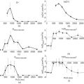
Figure 2.3 Example of measured C voxel(t), a reference AIF(t), and the fit (in red) of Eq. 2.5 to the data.
Related posts:
Stay updated, free articles. Join our Telegram channel

Full access? Get Clinical Tree


