Perfusion and Dynamic Contrast-Enhanced Imaging to Study Renal Function

Richard A. Jones

Shreyas Vasanawala

Damien Grattan-Smith

Renal Physiology

The kidneys receive approximately 25% of total cardiac input, which reflects the importance of the kidneys for waste excretion, electrolyte and acid-base balance, blood pressure homeostasis, and the resorption of essential nutrients. In a normal adult, approximately 600 to 700 mL/min of plasma flows into the renal glomeruli where a certain proportion of this plasma is filtered through Bowman’s capsule and the amount of filtrate per unit time is defined as the glomerular filtration rate (GFR). Substances that are not filtered at the glomerulus can still enter the urine by tubular excretion, while substances in the urine can reenter the circulation by tubular resorption.

GFR and renal plasma flow, which can be calculated from renal blood flow (RBF) by incorporating the patient’s hematocrit, are the two main parameters in the quantitative assessment of renal function. GFR varies with body size and can be normalized for body surface area. A normal measurement in young adults is approximately 120 mL/min per 1.73 m².¹ Approximate measurements of GFR can be derived from serum creatine levels using a standard formula such as the Modification of Diet in Renal Disease formula, however, they are affected by other factors, such as the muscle mass of the patient and his or her recent diet. Precise GFR measurement is not a trivial matter and has classically been calculated by measuring the clearance of a substance from the plasma that is neither secreted nor reabsorbed by the renal tubules. One substance that fits these criteria is the polysaccharide inulin, and measurements of the clearance of inulin have been regarded as the gold standard for GFR measurements for many years. However, inulin clearance measurements are time-consuming (because a steady state of inulin has to be established), expensive, have questionable reproducibility, are typically not available for routine clinical use, and only provide the total GFR rather than the GFR of the individual kidneys.

RBF is a measure of the volume of blood delivered to the kidneys per unit time and is closely related to renal plasma flow. Both GFR and RBF are altered in a variety of disease processes affecting the kidney. The ability to accurately and reproducibly quantify the GFR and RBF of each individual kidney in a single imaging session would greatly benefit the management of renal disease. Given that chronic kidney disease is one of the leading causes of death in the United States and accounts for over 8% of the Medicare/Medicaid budget, any technique that could provide reliable, quantitative values for RBF and GFR in a single imaging session would be of great value.

Pathophysiology

Renal diseases are typically classified as vascular, parenchymal, or combined. In any individual patient, there is a high degree of overlap of parenchymal and vascular disease. Perfusion imaging has the potential to provide a more complete evaluation of renal damage in patients with a wide variety of renal diseases including renal artery stenosis, urinary tract obstruction, renal transplant rejection, as well as a host of chronic renal diseases. In these conditions, noninvasive techniques are required to accurately measure various parameters of renal function and to monitor disease progression, establish a prognosis, and determine the optimal timing to initiate therapy.

The key toward understanding renal perfusion lies in the unique anatomic features of renal blood supply. The basic structure of the renal vasculature is shown in the upper panel of Figure 75.1. The main renal artery arises directly from the abdominal aorta and divides into multiple segmental arteries in the renal hilum. Accessory renal arteries arise from the aorta in 20% to 30% of normal people. The segmental renal arteries branch into a system of arching vessels called the arcuate arteries that run along the border between the renal cortex and renal medulla. From the arcuate arteries, the interlobular arteries arise at right angles and extend toward the surface of the kidney. The afferent arteriole of the glomerulus arises from branches of the interlobular artery. The efferent arteriole leads directly to the peritubular capillary circulation.

There are two separate capillary beds in the kidney: the glomerulus and the peritubular capillary bed. Both are shown in the lower panel of Figure 75.1. All the renal blood passes through both capillary beds. The capillaries of the glomerulus coalesce to form the efferent arteriole, which divides promptly into the peritubular capillary network. The pressure in the glomerular capillary bed is high (40 to 50 mm Hg), whereas the peritubular capillary bed has pressures similar to other capillary networks in the body, typically in the 5 to 10 mm Hg range. The peritubular capillaries coalesce to form the renal venous system. The blood supply to the renal medulla arises from the efferent arterioles in the juxtamedullary glomeruli via the vasa recta, which extend deep into the medulla alongside the renal tubules, forming tight hairpin bends.

FIGURE 75.1. Diagrammatic representation of renal vascularity and unique supply of the glomerulus and nephron. There are two distinct capillary networks in series that determine renal perfusion and glomerular filtration. The blood supply to the renal parenchyma is supplied by branches that arise distal to the glomerulus.

The renal cortex has ample blood supply that optimizes the GFR. The high capillary pressure in the glomerulus is the driving force for the glomerular filtration. The medulla is poorly oxygenated to preserve the osmotic gradients and enhance urinary concentration. The medulla concentrates urine up to four times the osmolality of plasma. To produce this unique gradient of osmolality, the medulla has a countercurrent system of the vasa recta and tubules, where sodium is actively reabsorbed in the setting of relative hypoxia. Renal medullary hypoxia is an obligatory part of the process of urinary concentration. For urinary concentration to occur optimally, an exact matching of oxygen supply and demand is required by precise regulation of the medullary blood flow and tubular work.

Although the kidney maintains function over a broad range of autoregulation, sustained reduction in renal perfusion leads to disturbed function at the microvascular level, vascular loss, and ultimately the development of interstitial fibrosis (Fig. 75.2). The chain of events that leads to renal injury is still a subject of research and varies among different diseases, but hypoxia and perfusion changes are invoked in most of the models. Additionally, RBF is known to change during many varied pathologic and pharmacologic stresses that influence renal function.² Decreased renal perfusion can trigger mechanisms that lead to progressive renal injury, whereas restoration of renal perfusion can positively influence the evolution of those mechanisms if it occurs prior to fibrosis. Nevertheless, once fibrosis is established, there is limited scope for the recovery of renal function.

Blood flow is different in the renal cortex and medulla and it is controlled by numerous mechanisms. The ability to separately study cortical and medullary perfusion could help us better understand renal pathophysiology in healthy individuals as well as patients with renal disease. There is a correlation between cortical and medullary blood flow that is predictable because the medulla receives its blood supply via the vasa recta that emanate from the cortical arterioles. To date, the main clinical application for renal perfusion measurements is in the qualitative assessment of renal artery stenosis. This is typically done using either contrast-enhanced or noncontrast (time of flight, phase contrast, inflow inversion recovery) angiography. Because the techniques used clinically for the evaluation of renal artery stenosis are discussed in standard clinical magnetic resonance imaging (MRI) textbooks, these will not be discussed in this chapter; rather, this chapter will concentrate on the measurement of renal blood flow.

Magnetic Resonance Imaging Techniques

Flow Measurements in the Renal Arteries

To date, the majority of renal flow measurements have been whole organ measurements that measured flow in the renal artery. Although this can provide valuable clinical information, it cannot provide any information on spatial variations in the RBF. Because this has been the dominant technique for 2 decades, a brief overview of the technique is given in the following section. The current standard for measurement of whole organ RBF with MRI is to use phase-contrast MRI to measure the blood flow in the renal arteries, because this has been shown to produce results that are comparable with those derived using the clearance of p–aminohippurate³ and the washout of xenon-133.⁴ To minimize the measurement errors, the technique is best performed using an imaging plane orthogonal to the renal artery, which necessitates that each renal artery is imaged separately. To minimize the effects of respiration, the images for each kidney are typically acquired during a breath-hold. The RBF is measured by calculating the flow within the aorta at multiple time points within the cardiac cycle and averaging these to obtain the mean flow velocity over the cardiac cycle. Multiplying this by the area of the region of interest used for the measurements gives the flow in milliliters per minute. The method requires several additional steps prior to the phase-contrast acquisition to determine the position of the renal arteries and hence accurately
position the phase-contrast MRI study to be orthogonal to the renal artery. Highly angled or tortuous renal arteries are technically difficult to assess for this reason. Failure to accurately position the slices can lead to a relatively large number of studies that cannot be evaluated.⁴ The cross-sectional area of the renal arteries must also be large enough to avoid partial volume effects, which generally prevent the application of the technique to pediatric patients. Note that the phase-contrast MRI-based flow measurement just gives a global measure of how much blood flows to the organ but does not allow one to assess the more interesting blood flow within the organ itself.

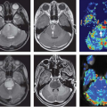
FIGURE 75.2. An 8-month-old boy with congenital hydronephrosis and severe uropathy of left kidney. (A) Axial T₂-weighted image shows a small left kidney with moderate hydronephrosis. The renal parenchyma is disorganized with loss of the corticomedullary differentiation. Innumerable small subcortical cysts are noted (B). Coronal T₁-weighted gradient-recalled echo (GRE) maximum intensity projection (MIP) image immediately after contrast administration demonstrates decreased enhancement of the left kidney. The nephrogram is poor. (C) Coronal T₁-weighted GRE source image during the nephrographic phase demonstrates decreased enhancement of the left kidney owing to microvascular damage and underlying renal dysplasia. (D) Coronal T₁-weighted GRE MIP image 15 minutes after contrast administration demonstrates excretion into the hydronephrotic left kidney. The renal parenchyma excretes but does not concentrate the contrast medium. (E) The signal intensity versus time curve is normal for the right kidney. The curve for the left kidney has a typical uropathic appearance with diminished perfusion and concentration in the renal parenchyma. After the initial relative decreased perfusion phase, the signal intensity curve for the left kidney concentration is less than the blood pool represented by the aortic curve, reflecting the fibrosis and microvascular damage that is known to occur in a uropathic kidney.

Dynamic Contrast-Enhanced Studies

In contrast to the measurements in renal arteries described previously, dynamic contrast-enhanced (DCE) studies can be used to provide spatial information for the RBF and the GFR. Much of the discussion on the measurement of flow in other chapters of this book has centered on DSC techniques (see Chapters 11 and 12); however, in the kidney, DCE imaging is preferred because this, in theory, allows for a quantitative measurement of both RBF and GFR. In addition, the quality of echo-planar imaging (EPI) images, routinely used for dynamic susceptibility contrast studies in the brain, is poorer in the abdomen than in the brain owing to increased susceptibility effects, which make them of little diagnostic value. This chapter will concentrate on elements of the data acquisition and analysis for DCE studies specific to renal studies. The ideal sequence for imaging renal function with MRI would have an excellent signal-to-noise ratio (SNR), be very fast, and be free from spatial distortion, and the signal changes induced by a gadolinium-based contrast agent (GBCA) would be linearly related to the concentration (amount)
of the GBCA. For renal studies, a gradient-recalled echo (GRE) sequence, with preparation pulses in some cases, is the most widely used sequence for DCE studies. The GRE sequence, while having minimal spatial distortion, offers lower SNR than an EPI sequence. The GRE sequence is also slower than EPI, which means that the desired spatial resolution, spatial coverage (number of slices), and temporal resolution cannot generally be obtained and compromises have to be made. In general, one or more techniques are used to accelerate the acquisition of the GRE data, and the reader is referred to Chapter 5 for a more detailed discussion of these techniques. Despite the use of these techniques, sufficient temporal resolution can be obtained only by acquiring a limited number of slices or, if whole kidney coverage is required, acquiring data with limited spatial resolution. The majority of studies of renal function to date have concentrated on measuring GFR, either because of hardware limitations, which restrict the available temporal resolution, or because the clinician wants to interrogate the dynamic images to determine if pathology, such as renal scarring, is present, which requires whole kidney coverage with higher spatial resolution. Figure 75.3A shows an example of DCE images acquired for a patient with relatively normal anatomy and function. Although the theme of this chapter is renal perfusion, it is generally desirable to
measure both the GFR and RBF when using a GBCA; so some discussion of the methods used for measuring the GFR is included here because the same data can be used to measure the RBF if the temporal resolution is sufficiently high.

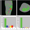
FIGURE 75.3. (A–C) Show the same slice from three volume acquisitions acquired at time points corresponding (from left to right) to the cortical (arterial), parenchymal, and excretory phases of renal function, respectively. (D–F) Maximum intensity projections derived from the total volume for the three same time points. (G) on the left, the arterial and parenchymal time-intensity curves are shown. The curves are expressed in terms of the relative signal (RS), which is calculated using the signal at each time point, S_t, and the mean precontrast signal (S₀) using the expression RS = (S_t − S₀)/S₀ and is linear related to the contrast agent concentration up to contrast agent concentrations of approximately 1 mmol/L for the sequence parameters used in the study. Hydration and the administration of Lasix (furosemide) 15 minutes prior to contrast injection were used to ensure a high urine output. on the right, the curves were fitted to the Annet model. The upper curves show the overall fit in green with the measured curve being shown in red. The lower panels show the vascular (cyan) and parenchymal (yellow) components of the fit.

As discussed in Chapter 23, GBCAs shorten both the T₁ and T₂ relaxation times, and there is a linear relationship between the relaxation rate and the concentration, c, of the GBCA at time t, which, for T₁, can be expressed as:

where r₁ is the T₁ relaxivity of the GBCA at time t and T₁₀ is the native T₁ (i.e., in the absence of the GBCA). The expression for T₂ is analogous with r₂, T₂, and T₂₀, replacing r₁, T₁, and T₁₀. Taking standard values for the T₁ and T₂ relaxivities of a GBCA (r₁ = 4.5 mM⁻¹ s⁻¹, r₂ = 5.5 mM⁻¹ s⁻¹) and typical values for the relaxation times of the renal cortex at 1.5T,⁵ then the effect of a 0.5 mM concentration of a typical GBCA would be to induce a threefold reduction in T₁ (from 880 to 295 milliseconds), while T₂^* would change by only 15% (from 66 to 56 milliseconds). Thus, the GBCA produces a far larger change in T₁ than in T₂. The spoiled GRE achieves T₁ weighting by using a short repetition time, a relatively high flip angle, and a short echo time (to minimize T₂^* effects) in conjunction with techniques (spoiling) to prevent any transverse magnetization from being refocused by subsequent radiofrequency pulses. When using a GRE sequence with a short repetition time (TR) and echo time (TE), the effect of T₂^* shortening is often assumed to be negligible (i.e., TE ≪ T₂^*) for the concentrations of GBCAs encountered in vivo. However, it should be noted that relatively high concentrations occur in the blood during the first passage of the GBCA. In addition, the concentrating function of the kidney results in progressively higher concentrations as the GBCA passes through the kidney, leading to elevated concentrations in the distal tubules and collecting ducts. In addition to the potential loss of the signal originating from within these structures because of T₂^* shortening, there is also the possibility that an inhomogeneous distribution (i.e., present within these structures but absent from the surrounding tissue) of a highly concentrated GBCA can generate a susceptibility effect (see Chapters 11 and 12 for more details of this mechanism). This effect is analogous to the blood oxygen level–dependent effect used in functional MRI studies but with an exogenous agent (i.e., the GBCA), rather than an endogenous agent (blood) generating the effect. Here, the T₂^* shortening leads to a reduction, rather than an increase, in the signal in the surrounding renal tissue. Methods used to reduce the concentration of the GBCA in the tubules and collecting ducts include hydration of the patient and use of a diuretic agent, such as furosemide, prior to the injection of the GBCA.⁶ These interventions will induce a high urine output state where proportionately more urine volume will be generated for a given amount of a filtered GBCA.

A uniform flip angle over the slice is also often assumed when deriving the contrast agent concentration from the MRI signal. Although this is a reasonable assumption for the central slices of a three-dimensional volume, it is not appropriate for images acquired as a two-dimensional slice because the flip angle will vary across the slice and this has to be taken into account by integrating the signal across the slice profile. Additionally, because the slice profile is also a function of T₁, the slice profiles of the pre- and postcontrast studies will not necessarily be the same. Furthermore, for higher field strengths (e.g., 3T and higher), a considerable spatial variation of the transmit B1 field can be observed. This in turn can lead to a corresponding variation of the flip angle and, thus, errors in calculations of the tracer concentration. A detailed discussion of these and other issues that can complicate the analysis of DCE data is given in Chapters 23 and 29.

Only gold members can continue reading. Log In or Register to continue