Perfusion Imaging in Liver and Pancreas

Se Hyung Kim

Dow-Mu Koh

Jürgen K. Willmann

Liver

The assessment of the liver is an essential component of abdominal oncologic imaging for both the detection of metastatic disease and the diagnosis of primary hepatic tumors such as hepatocellular carcinoma (HCC) because the liver is the second most common site of metastatic disease¹ and hepatocellular carcinoma (HCC) is the fifth most common cancer in the world, responsible for up to 1 million deaths annually worldwide.² The diagnosis and follow up of liver tumors using current imaging methods primarily rely on the morphologic changes of the tumors compared with normal surrounding liver tissue. For example, morphologic criteria used in the diagnosis of liver metastasis on conventional computed tomography (CT) or magnetic resonance imaging (MRI) are lesions showing low attenuation (or low T₁ signal intensity) with or without peripheral hyperenhancement on contrast-enhanced portal venous phase images; and nodules showing hypervascularity on arterial phase, associated with washout on portal venous or equilibrium phase images for HCC (Fig. 65.1). Although imaging techniques such as ultrasound (US), CT, and MRI are commonly used for the detection of liver tumors, the limitations of a morphologic feature-based approach are well recognized.³^,⁴ Conventional imaging techniques allow diagnosis of most liver tumors over 1 cm (sensitivity of 55% to 90%), however, the sensitivity for smaller lesions (≤1 cm) is much lower (<50%) and microscopic lesions remain occult.³^,⁴^,⁵^,⁶

In addition to accurate diagnosis, early detection of liver tumors, predicting prognosis based on imaging criteria, and accurate assessment of tumor response to novel therapies also present great challenges for oncologic imaging. Novel therapies often show no or only late effects on tumor size, and current Response Evaluation Criteria in Solid Tumors (see Chapter 56) criteria may not adequately assess the response to novel targeted treatments.⁷^,⁸ Furthermore, early cancer detection is critical to improve patient survival. For example, the 4-year survival rate in patients with cirrhosis and HCCs, who met the predetermined criteria for liver transplantation, was 85% among patients who underwent liver transplantation⁹; whereas the prognosis of patients with advanced, symptomatic HCC was dismal, with a 5-year survival rate of less than 5%.¹⁰ This discrepancy suggests that early detection of small HCC is critical for better patient outcomes. Similarly, early detection of liver metastasis and confident assessment of early tumor response to treatments are also critical for optimized patient management. Early detection of poor treatment response may allow a rapid switch to alternative therapeutic strategies, thereby minimizing unnecessary costs and potential side effects and providing a more individualized therapy.¹¹

FIGURE 65.1. Characteristic contrast-enhanced computed tomography (CT) findings of hepatic malignancies. (A) Hepatic metastases from pancreatic adenocarcinoma in a 79-year-old woman. Arterial (left) and portal venous (right) phase CT images show two poorly demarcated low attenuating lesions (arrows) in both hepatic lobes. Note peripheral rim-like enhancement (arrowheads) shown in both lesions during arterial phase imaging. (B) Hepatocellular carcinoma in a 64-year-old male hepatitis B carrier. on arterial (left) phase CT image, a peripheral, well-demarcated hypervascular mass (arrow) is seen in liver segment VIII. on portal venous (right) phase, the mass appears hypodense (washout) compared with surrounding liver parenchyma.

To further improve our ability to better diagnose and monitor liver tumors, functional imaging techniques, such as perfusion CT or perfusion MRI have been developed in recent years. Perfusion imaging is attractive because it has the potential to detect tumors earlier by
demonstrating global and regional alterations of blood flow, which usually precede morphologic changes.¹²^,¹³^,¹⁴ More specifically, in the liver, perfusion imaging allows for detection of primary and metastatic tumors earlier by resolving hepatic arterial and portal venous components of blood flow on a global and regional basis. Thereby, it allows for potential improvement in the earlier detection of liver lesions.¹²^,¹³^,¹⁴ However, the liver is one of the most challenging organs for perfusion imaging because of considerable nonuniform motion during respiration and its unique dual vascular supply.

The first part of this chapter reviews the perfusion physiology of the liver, methods for quantitative analysis by perfusion CT and MRI, and currently available data that support the use of these techniques in preclinical and clinical applications.

Physiology and Structural Basis for Liver Perfusion

The liver is a highly vascularized organ that is predominantly supplied by the low-pressure portal vein (75%) and supplemented by the high-pressure hepatic artery (25%).¹⁵ The two vascular inputs mix in porous vascular channels (sinusoids), which eventually empty into the central venous system (Fig. 65.2). Between the sinusoids and a row of hepatocytes there is a small space (called space of Disse), which may be considered an interstitial space (Fig. 65.2). Unlike other organs, discontinuity of sinusoidal endothelium through the fenestrae facilitates the transport of low molecular-weight compounds (such as iodinated CT or low molecular weight gadolinium MR contrast agents) between the intravascular space (sinusoids) and the interstitial space (space of Disse) in the liver.¹² The sinusoids represent almost one-third of the volume of the liver parenchyma, whereas the space of Disse constitutes only 10% of the total liver volume.¹³ Free exchange of contrast agents between these two spaces through fenestrae occurs in the normal liver, providing the rationale to use a single compartment pharmacokinetic model for liver perfusion imaging in a number of clinical scenarios.

FIGURE 65.2. Diagrams showing microscopic anatomy of the liver. (A) Blood from both hepatic artery and portal vein mixes together in the sinusoids and then drains out of the hepatic lobule through the hepatic vein. (B) The sinusoids are lined with fenestrated endothelial cells, with no basement membrane. The fenestrations permit blood plasma to flow freely into the interstitial space between sinusoids and hepatocyte cords. This space is called the space of Disse. Stellate cells, which regulate blood flow through the liver, are located within the space of Disse. (A: Modified from Jarnagin WR. Liver and portal venous system. In: Doherty GM, ed. Current Diagnosis and Treatment: Surgery. 13th ed. New York: McGraw-Hill; 2010:509–543; B: Modified from Prudêncio M, Rodriguez A, Mota MM. The silent path to thousands of merozoites: the plasmodium liver stage. Nat Rev Microbiol. 2006;4:849–856.)

To maintain a stable blood supply to the liver, the total hepatic blood flow is finely controlled by the so-called hepatic arterial buffer response, which is the inverse response of the hepatic artery to changes in portal venous flow.¹³^,¹⁶ The buffer response is mediated largely by local concentration of the vasodilator adenosine. Adenosine is produced at a constant rate in a fluid-filled space (called space of Mall) within the portal triad surrounding the hepatic arterioles and portal venules.¹⁷ Adenosine can either diffuse into the portal vein through sinusoids and be washed away or it can remain locally and act on adenosine receptors on the hepatic artery, causing vasodilatation.¹⁸^,¹⁹ With decreasing portal venous flow, adenosine accumulates and leads to hepatic arterial vasodilatation, therefore, higher blood supply via the hepatic artery compensates for the decreased portal venous supply. However, portal venous flow does not increase with reductions in hepatic arterial flow.

Computed Tomography Perfusion versus Magnetic Resonance Perfusion

A variety of imaging techniques have been used to measure perfusion parameters in the liver. They include flow scintigraphy using technetium 99-labeled radiopharmaceutical agents, Doppler US,
contrast-enhanced US, positron emission tomography (PET) using oxygen-15-labeled water ([¹⁵O]H₂O) tracer, CT, and MRI. Among them, CT and MRI are the two most commonly used modalities for clinical perfusion imaging because of recent technological advances and because both modalities are already routinely used for monitoring cancer patients (in particular CT). Regardless of the modality used (i.e., CT or MRI), the fundamental steps for perfusion imaging are the same and include intravenous injection of contrast agents, dynamic time-resolved image acquisition, pharmacokinetic modeling, analysis, and interpretation of perfusion parameters. However, there are several differences between CT- and MR-based perfusion imaging. First, different types of contrast agents are used (i.e., nonionic iodinated agents for CT and low molecular weight gadolinium chelates for MRI). Furthermore, CT and MRI have fundamentally different principles of image acquisition. Although both CT and MRI contrast agents have similar molecular weights, their pharmacokinetics can vary in the same patient because of differences in molecular charge, configuration, and protein affinity binding. Thus, both contrast agents can have different kinetic behavior in the examined tissue. Also, unlike MRI, the degree of contrast enhancement expressed as the Hounsfield unit (H) on CT is linearly related to contrast agent concentration and is independent of the microenvironment present at the tissue level, which makes mathematical modeling for CT perfusion straightforward and relatively simple when compared with that of MR perfusion imaging.²⁰^,²¹ In MRI, the measured T₁ signal intensity does not scale linearly with gadolinium concentration, which means that calibration of tissue T₁ relaxation time is necessary for the accurate quantification of gadolinium contrast kinetics in tissues. Other advantages of CT perfusion include a high temporal resolution (approximately <0.5 s) for monitoring contrast agent in the first pass, wide availability, relatively low cost of CT, ease of standardization, and ease of incorporation into standard CT protocols for staging and therapeutic assessment of patients.²² Both MR and CT perfusion imaging have moderate to good reproducibility in the liver, especially in the hands of expert centers, but CT can have better patient acceptability.²³^,²⁴^,²⁵ Nevertheless, although current MR technology might have a lower temporal resolution in comparison with CT perfusion imaging (which may influence the accuracy of first-pass kinetic estimations), the absence of ionizing radiation means that the acquisition time can be stretched over a longer period of time for delayed permeability imaging, while the use of ionizing radiation on CT imposes a limit on the total number of scans. The lack of radiation burden also means that perfusion MR studies may be repeated more frequently than CT to track serial vascular changes following treatment. Other advantages of MRI include higher sensitivity of MRI to gadolinium chelate agents than CT using iodinated contrast agents, the relatively high signal-to-noise ratio (SNR) of three-dimensional volumetric MR acquisition (compared with thin-section CT), and the potential to combine perfusion measurements with other quantitative MRI techniques, during the same imaging session, such as diffusion-weighted imaging.²⁶

Dual Vascular Input in Liver Perfusion Imaging

The liver is one of the most challenging organs for perfusion imaging because of its considerable nonuniform motion during respiration, its large size, and its unique dual vascular supply. Although postprocessing motion-compensation techniques and increased field-of-view imaging with the latest generation CT scanners can address issues with tissue motion and organ size, the dual vascular supply of the liver from both the hepatic artery and portal vein makes the application of perfusion imaging to the liver challenging. Some researchers propose the use of a single-input model for perfusion imaging of hepatic metastases with the assumption that the vascular supply is predominantly arterial, although this assumption may not be true for all metastases.²⁷^,²⁸ Indeed, Liu et al.²⁹ showed that the proportion of arterial and portal venous blood supply to the liver metastases can change as the tumor grows. They also showed in a murine metastasis model using a colonic adenocarcinoma cell line that intratumoral microcirculation varies from direct diffusion, to portal perfusion, to mixed portal and arterial perfusion, and finally, to predominantly arterial perfusion in accordance with stepwise tumor neovascularization during the growth of hepatic metastases. Likewise, Koh et al.³⁰ also demonstrated significant portal perfusion in hepatic metastasis of three patients with colon or ovary cancer using a dual-input, dual-compartment model on MR perfusion. Therefore, the separation of hepatic arterial and portal blood supplies in normal liver tissue and liver lesions is important for proper interpretation of the liver perfusion parameters because the absolute and relative changes of dual vascular supply can provide additional information for better detection, characterization, prognostication, and treatment monitoring of the liver disease. However, direct measurement of the portal input function can be challenging on MRI, especially in the presence of motion.

Definition of Perfusion Parameters

CT and MR perfusion imaging provide absolute and relative information about tissue or tumor perfusion parameters such as blood flow (BF, F), blood volume (BV, V_b), mean transit time (MTT, T_m), permeability surface area product (PS), and extraction fraction (E). BF is the volume flow rate of blood through the vasculature and is expressed as milliliters per minute per 100 mL. BV is the
volume of blood within the vasculature that is actually flowing and is expressed in units of milliliters per 100 mL. MTT is the time taken for the blood to traverse between the arterial inflow and the venous outflow, which is measured in seconds. PS is the product of permeability and the total surface area of the capillary endothelium in a unit mass of tissue or tumor, which is measured as milliliters per minute per 100 mL. E is the fraction of solutes present in arterial inlets, with the potential to diffuse into the interstitial space, which actually becomes transferred from blood to the extravascular-extracellular space (EES) during a single passage of blood from the arterial end to the venous end of the capillaries of a tumor. K^trans used for MR perfusion imaging is a volume transfer constant between blood plasma and the EES. In high-permeability situations, where flux across the endothelium is flow-limited (a common situation in tumors), the transfer constant is equal to the blood plasma flow per unit volume of tissue.³¹ In cases of low permeability, where tracer flux is permeability limited (usually in normal tissues), the transfer constant is equal to the PS between blood plasma and the EES, per unit volume of tissue.³¹

Maximum Slope Model

When using the maximum slope model, where tissue perfusion is determined via dividing the peak enhancement gradient of the tissue on the time-density (CT) or time-contrast concentration to time-signal intensity (MRI) curve by the peak aortic enhancement, the separation of arterial and portal components in regions of interest of the liver can be obtained by assuming that maximum splenic enhancement marks the end of the arterial phase and the beginning of the portal venous phase of liver perfusion.³²^,³³^,³⁴^,³⁵ To calculate both arterial and portal perfusion (F_a, F_p) of the liver, the following equations are used:

The equations state that tissue arterial (F_a) perfusion (or tissue portal [F_p] perfusion) is the ratio of the maximal rate of accumulation of contrast in tissue or the maximum slope of Q(t) to the maximum arterial [C_a(t)]_max (or portal [C_p(t)]_max) concentration at a given time. In the liver, the maximal slope of the liver time-density curve (time-signal intensity or time-contrast concentration curve on MRI), [dQ(t)/dt]_max, in each phase (arterial and portal venous, respectively), is divided by the peak aortic ([C_a(t)]_max) and portal ([C_p(t)]_max) enhancement to calculate both arterial and portal perfusion, respectively.³⁴^,³⁵^,³⁶^,³⁷ Furthermore, the hepatic perfusion index (HPI), which is the ratio of the arterial perfusion to the total hepatic perfusion (HPI = arterial perfusion/arterial + portal perfusion), can also be calculated.³²^,³³ Totman et al.³⁸ and Miyazaki et al.³⁹ adapted the maximum slope model to gadolinium-enhanced MR perfusion and reflected hepatic dual vascular supply on the measurement of HPI by separating arterial flow from portal flow according to the time of peak splenic enhancement. Although this slope-ratio technique is simple to implement, it does not give information regarding other perfusion parameters, such as BV, MTT, or capillary PS. This is because it takes into account only the rising part (first pass) of the liver enhancement curve before the venous outflow.¹³ Furthermore, to satisfy the no venous outflow assumption, a relatively high injection rate (15 to 20 mL/s) has to be used in CT and an injection rate of 3 mL/s or greater is recommended for MRI.

Tracer Kinetic Models

To avoid the approximations of the arterial and portal slopes and to obtain other perfusion parameters, tracer kinetic modeling techniques, such as the compartment model and the deconvolution model, have been developed.⁴⁰^,⁴¹ Patlak et al.⁴² and Patlak and Blasberg⁴³ proposed the use of compartmental models to describe the distribution of blood-borne solutes in tissue, enabling simultaneous measurement of other perfusion parameters. Because contrast agents are usually inert, the distribution of contrast agents in tissue calls for only two compartments: the intravascular (plasma) space and the interstitial space. They assumed that the intravascular space is a well-mixed compartment in which the solute concentration is spatially uniform. In other words, there is no concentration difference within the vasculature of tumors. This model was simplified to the Patlak plot by adapting another assumption that there is no back flux of contrast agent from the interstitial to the intravascular space,⁴²^,⁴³ as shown in the equation:

where Q(t) is tissue concentration along the time, C_a(t) is arterial concentration along the time, FE is the transfer constant of contrast agent, V_b is a blood volume within the vasculature in a tumor. If Q(t)/C_a(t) is plotted versus

, the result is a straight line, with a slope of FE and an intercept of V_b.⁴⁴ Nevertheless, the Patlak plot has several limitations. First, there is the no backflow assumption, which will not be valid in all tissues. Second, in real situations, there is a concentration gradient from the arterial to the venous end of capillaries as blood travels down the length of capillaries and contrast material partially leaks out. Third, blood flow (F) and extraction fraction (E) cannot be measured separately because they are determined together as the transfer function (FE).⁴⁴ Except when E is known to be close to 1, FE is not an absolute measure of tumor perfusion.

To reflect the unique dual input system of the liver, Materne et al.⁴⁵ and Van Beers et al.⁴⁶ have proposed a dual-input, single compartment model:

where Q(t), C_a(t), and C_p(t) are the contrast agent concentrations measured over time, respectively, within the liver tissue, hepatic artery, and portal vein derived from regions of interest drawn over liver parenchyma, abdominal aorta, and main portal vein, and k₁_a, k₁_p, and k₂ are the arterial and portal venous inflow and liver outflow (hence the “–” sign) rate constants.¹³ By fitting measured Q(t), the constants k₁_a, k₁_p, and k₂ can be estimated and can be used to calculate hepatic arterial and portal venous perfusion, MTT of contrast agent through the liver, and contrast agent distribution volume within the liver (V_d). The V_d of contrast agent is used instead of the hepatic BV because iodinated contrast agent used in CT leaks freely and instantaneously across the sinusoidal wall, which leads to a distribution volume that associates the hepatic BV with part of interstitial space (space of Disse).¹³ This dual-input compartment model also assumes that there is an instantaneous mixing of blood in the capillary (intravascular) component, inevitably causing limitations in the Patlak model.

The most commonly used compartment models for MR perfusion parameter measurements are the Tofts⁴⁷ model and Larsson et al.⁴⁸ model, which are bidirectional and dual-compartment models. These models are considered to partially solve the limitations of the Patlak model in CT perfusion imaging by reflecting both fluxes between intravascular and extravascular spaces. But neither models addresses the dual blood supply of the liver. Materne et al.⁴⁹ first took the dual arterial and portal venous input of the liver into account for MRI measurements of hepatic perfusion parameters by adapting their compartment CT perfusion model to validate the accuracy of MR perfusion parameter using radiolabeled microspheres in normal rabbits. Several researchers, including Annet et al.⁵⁰ and Hagiwara et al.⁵¹, and Miyazaki et al.⁵² used the MR model from Materne et al. and investigated perfusion changes in diffuse liver disease and focal liver lesions. Table 65.1 summarizes protocols of data acquisition and contrast administration and kinetic models of liver MR perfusion.

The main motivation for the development of noncompartment models is to enable the separation of F (tumor perfusion) and E (or permeability surface area product). It is possible for these models to separate them because they do not assume that the intravascular space is a compartment with a spatially uniform solute concentration. Indeed, the capillary network is complex and the MTT is long in the liver, where this assumption does not work significantly. Since the simplest distributed parameter model was first proposed by Johnson and Wilson,⁵³ Axel⁵⁴ has introduced the deconvolution method into functional CT by calculating tissue MTT. Supposing that the concentration–time curve is known both at the arterial inflow and at the venous outflow, a transfer function specific to the tissue can be measured, enabling the calculation of the perfusion parameters of the tissue. But because the concentration–time curve at the venous outflow of the tissue cannot be measured, we have to infer the venous outflow concentration–time curve from both concentration–time curves of the arterial inflow (input function) and the tissue using the concept of impulse residue function.¹³ The concentration–time curve of a contrast agent remaining within the tissue C_t(t) can be predicted for any type of input function, C_i(t) and tissue residue function, R_t(t) as the convolution of C_i(t) by R(t),¹³ as shown in the equation (see Chapters 24 and 25):

A deconvolution process can allow the determination of R(t), knowing the contrast concentration–time curve of the tissue C_t(t) and the input function C_i(t). If we can calculate residue function of the tissue R(t), the output function C_o(t) can also be calculated.¹³ Using this, other kinds of perfusion parameters can be calculated. For instance, blood flow (F) is calculated as the initial (maximal) value of R(t), that is, R(t = 0). The MTT can be calculated as the first moment of the calculated C₀(t), as shown in the equation:

Finally, distribution volume of the contrast within the tissue (blood volume) is measured by multiplying F and MTT using the central volume theorem,¹³ as shown in the equation:

Deconvolution methods are appropriate for measuring lower levels of perfusion (<20 mL/min/100 mL) because they are able to tolerate greater image noise attributable to the inclusion of the complete time series of images for calculation.⁵⁵ This is particularly beneficial for the accurate measurement of lower perfusion values, typically seen in tumors after treatment response.⁵⁵ Nevertheless, a potential drawback of this method is the possibility of image misregistration, secondary to motion of the patient because it needs all the acquired images for calculation.

For liver perfusion imaging, Cuenod et al.⁵⁶^,⁵⁷ and Fournier et al.⁵⁸ proposed a specific deconvolution technique. The characteristic features of the liver for their approach come from its dual vascular input, although they used a single-compartment model. In the liver, arterial and portal bloods are mixed in the sinusoidal capillaries and the tissue concentration–time curve in the liver (referred to as Q) can be expressed as:

where α is the hepatic perfusion index and R(t) is the tissue residue function over time after contrast administration.
A deconvolution program can allow the determination of R(t) and α (hepatic perfusion index) because we know the contrast concentration–time curve of the liver Q(t) and the input function of both hepatic artery C_a(t) and portal vein C_p(t). R(t) allows the calculation of C₀(t), MTT as the first moment of the calculated C₀(t), and F_T (total blood flow) as the initial (maximal) value of R(t) [=R(t = 0)]. V_d is measured by multiplying F_T and MTT using the central volume theorem. Finally, arterial and portal blood flow can be calculated using F_T and α (hepatic perfusion index), as shown in the equation:

Abdullah et al.⁵⁹ and Koh et al.³⁰ reflected hepatic dual vascular supply on MR perfusion imaging by simply adapting dual-input CT deconvolution model, proposed by Cuenod et al.,⁵⁶ although Koh et al. proposed a dual-compartment version of deconvolution MR model to describe the tracer behavior in hepatic metastasis.

TABLE 65.1 SUMMARY of DATA ACQUISITION AND POSTPROCESSING METHODS of HEPATIC MAGNETIC RESONANCE PERFUSION FROM LITERATURE REVIEWS

Author	Journal/Year	Acquisition Parameters		Gadolinium Contrast Agent		Latest Scan Time (s)	SI Conversion to Gd Concentration^a	Analysis Method
Author	Journal/Year	Tesla of Scanner	Sequence	Type/Amount (mmol/kg)	Injection Rate (mL/s)	Latest Scan Time (s)	SI Conversion to Gd Concentration^a	Model	Input/Compartment
Totman et al.³⁸	Br J Radiol/2005	1	3D FSPGE	Magnevist/0.1	4	75	No	Maximum slope	Dual/single
Miyazaki et al.³⁹	Eur Radiol/2008	1.5	2D FSPGE	Magnevist/0.1	3.5	420	Yes	Maximum slope	Dual/single
Wang et al.¹⁰²	AJR/2004	1.5	2D FLASH	Omniscan/0.15	2.5	79	No	Qualitative^b	Not applicable
Morgan et al.²⁷	JCO/2003	1.5	Turbo FLASH	Magnevist/0.1	NA	300	Yes	Compartment	Single/dual
van Laarhoven et al.²⁸	JMRM/2003	1.5	2D FLASH	Magnevist/≈0.1	2.5	90	No	Compartment	Single/dual
Materne et al. ⁴⁹	Magn Reson Med/2002	1.5	2D FSPGE	Dotarem/0.05	NA	NA	Yes	Compartment	Dual/single
Annet et al.⁵⁰	Radiology/2003	1.5	2D FSPGE	Dotarem/0.05	3	NA	Yes	Compartment	Dual/single
Hagiwara et al.⁵¹	Radiology/2008	1.5	3D FSPGE	Magnevist/≈0.05	5	120	Yes	Compartment	Dual/single
Johnson et al. ⁸³	ISMRM Proc/2008	1.5	3D FSPGE	Magnevist/≈0.05	NA	NA	Yes	Compartment	Dual/single
Abdullah et al.⁵⁹	JMRI/2008	1.5	2D FSPGE	Dotarem/0.1	4	85	No	Deconvolution	Dual/single
Xu et al.⁸⁹	JMRI/2008	1.5	2D FLASH	Magnevist/0.1	0.5	120	No	Qualitative^c	Not applicable
Koh et al.³⁰	Radiology/2008	1.5	3D FSPGE	Omniscan/0.2	3	320	Yes	Deconvolution	Dual/dual
Miyazaki et al.⁵²	Radiology/2012	1.5	3D FSPGE	Magnevist/NA	3	240	Yes	Compartment	Dual/single
SI, signal intensity; 2D, two-dimensional; 3D, three-dimensional, FSPGE, fast spoiled gradient echo; FLASH, fast low angle shot; NA, not available. ^a Magnetic resonance signal intensity was converted to gadolinium concentration using T₁ mapping. ^b Peak enhancement, maximum enhancement, and enhancement slope percentage were calculated from time-intensity curves in first-pass studies. ^c Relative signal enhancement (%), time-to-peak, and initial slope of enhancement were calculated from time-intensity curves.

Acquiring Perfusion Images (see Appendix)

Image Acquisition Protocol

Computed Tomography Perfusion

Figure 65.3 presents all of the steps for CT perfusion from CT data acquisition to postprocessing methods. Various kinds of perfusion CT protocols have been proposed, typically depending on the target organ, pharmacokinetic modeling, CT scan configuration, and clinical purpose.¹⁴ Nevertheless, a typical perfusion CT protocol comprises acquisition of unenhanced CT, followed by a dynamic acquisition performed sequentially after intravenous injection of contrast agent.⁵⁵ The dynamic image

acquisition includes a first-pass study, a delayed study, or both, depending on the pertinent physiologic parameter that needs to be analyzed.⁵⁵

FIGURE 65.3. Steps involved in a computed tomography (CT) perfusion examination of liver metastasis from colon cancer in a 46-year-old woman. (A) First, an unenhanced image and a series of dynamic images following administration of contrast agent are acquired. Numbers in left lower corner represent the time from injection of contrast agent. (B) After loading the perfusion CT dataset on a workstation with dedicated perfusion CT software, motion correction using either rigid or nonrigid registration methods is performed for anatomic alignment. (C) After motion correction, a region-of-interest (ROI) within the proximal abdominal aorta is drawn to obtain an arterial input function (AIF) (red circle in upper left image). Furthermore, for liver perfusion imaging, a second ROI is drawn within the portal vein to determine portal venous input function addressing the unique character of dual blood supply in the liver (not shown). A third ROI is drawn over the spleen, which allows separation of arterial and portal venous blood flow in the liver (green in upper right image). Note, time-density curves were generated from the abdominal aorta (red), the portal vein (blue, not shown in CT image), and the spleen (green). The yellow curves represent normal liver tissue. (D) The perfusion software automatically generates color-coded perfusion maps of the entire liver representing blood flow (BF), blood volume (BV), permeability, hepatic arterial perfusion (HAP), portal venous perfusion (PVP), and hepatic perfusion index (HPI). Note, in this example, an increased HPI in several liver metastases can be already appreciated by visual inspection (arrows). (E) After drawing additional ROIs over liver lesions (e.g., in this example a metastasis [ROI 1] and normal liver tissue [ROI 2]), quantitative perfusion parameters are displayed. Note that in this example all CT perfusion parameters except HPI obtained in the liver metastasis (ROI 1) show lower values than those of adjacent normal liver parenchyma (ROI 2).

The baseline unenhanced CT acquisition should provide wide coverage to include the organ of interest. This study basically serves as a localizer to select the appropriate tissue area to be included in the dynamic contrast-enhanced (DCE) imaging range. Depending on the scanner configuration, a 2-cm coverage area (for a 4- or 16-row CT scanner) or a 4-cm coverage area (for a 64-row CT scanner) can be selected for dynamic scanning. Larger coverage (8 to 16 cm) is now feasible with the availability of newer scanners with 128 to 320 rows of detectors or with a dynamic four-dimensional spiral scan mode, which allows for the extension of the z-axis coverage beyond the width of the scanner detector.¹⁴^,⁶⁰

The first-pass study for perfusion measurements comprises images acquired in the initial cine phase for a total of approximately 40 to 60 seconds. For the typical first-pass study, image acquisition is done every 1 to 5 seconds,
depending on pharmacokinetic modeling used.⁵⁵^,⁶¹^,⁶² For obtaining permeability measurements, second phase images are acquired every 10 to 20 seconds for 2 to 10 minutes after the first-pass study.⁵⁵^,⁶² For both first-pass and delayed studies, a deconvolutional method usually requires images with higher temporal resolution (i.e., every 1 second for first-pass study and every 10 seconds for delayed study) than the compartment models (every 3 to 5 seconds for first-pass study and every 10 to 20 seconds for delayed study).⁵⁵^,⁶¹^,⁶²

The mathematic modeling technique employed also has implications on the CT protocol used. Deconvolution methods are appropriate for measuring lower levels of perfusion (<20 mL/min/100 mL) because they can tolerate greater image noise attributable to the inclusion of the complete time series of images for calculation.⁵⁵ Nevertheless, a potential drawback of including all the acquired images for calculation is the possibility of image misregistration secondary to motion of the patient.⁵⁵ Therefore, the deconvolution method allows the use of a lower tube current (50 to 100 mAs) and permits scanning with higher temporal resolution for the dynamic cine acquisition.¹⁴^,⁵⁵^,⁶² Conversely, compartmental analysis effectively uses fewer images for perfusion measurement. Therefore, patient motion has relatively less impact on the analysis.⁵⁵ The presence of image noise results in miscalculation of perfusion values for the compartment modeling; therefore, a higher tube current (100 to 250 mAs) with lower image frequency is usually preferred for CT perfusion analyzed using the compartmental method.¹⁴^,⁵⁵^,⁶² For the tube voltage, 80 kVp rather than 120 to 140 kVp not only reduces the administered radiation dose by a factor of three or more but also increases conspicuity of intravenous contrast agent. The latter is partly because the mean photon energy (43.7 KeV) for 80 kVp photons is much closer to the K-edge (33.2 KeV) of the iodine within the contrast agent.⁶³ In addition, although there is a linear relationship between H and iodine concentration, regardless of the peak kilovolt settings, the slope of H versus iodine concentration is the steepest on 80 kVp. Therefore, 80 kVp is considered the optimal peak kilovolt to be used in CT tumor perfusion imaging of the liver and pancreas.

Magnetic Resonance Perfusion

Because of the nonlinear relationship between blood gadolinium concentration and MR signal intensity, an additional step is required for MR perfusion to convert the MRI signal [SI(t)] to gadolinium concentration [c(t)] and eventually to measure the perfusion values of the organs or tumors in meaningful units (i.e., milliliters per minute per 100 mL). Conversion can be possible by the step of generating a native tissue T1 map (T10) before obtaining DCE-MRI (see Chapter 23). One common method of measuring tissue T10 value is to acquire multiple gradient echo T1-weighted images with variable flip angles. The pulse sequence and coils used for T1 calculation should be the same used for DCE-MRI protocol. Keep in mind, although, that this method heavily depends on the underlying transmit B1 field and exact knowledge of the applied flip angle. Any spatial deviation of B1 will cause errors in the estimation of T10. Alternative T10 mapping methods, based on saturation recovery or inversion recovery principles, are sometimes preferable. Prior to contrast arrival, several baseline acquisitions (typically five) are recommended to obtain stable and high SNR images for baseline signal intensity [SI(0)] measurement (steady state).⁶⁴ Because normalization to the baseline signal is usually performed, a good estimate of the baseline is recommended. The latter improves with the number of baseline images that are averaged together. Because the T10 mapping process is adding extra scan time and may generate noisy estimates that are then propagated in the perfusion analysis (increase noise in perfusion estimates), several researchers have skipped T10 mapping under the assumption that the measured signal intensities on MRI are linearly correlated to gadolinium concentrations.⁶⁵ This may affect the accuracy of results because the optimal approach is highly dependent on the pulse sequences, MR scanners, and range of gadolinium concentrations encountered during MR acquisition.⁶⁵ After precontrast series to measure a T10 map have been acquired, a dynamic acquisition is performed sequentially after intravenous injection of contrast agent using a two-dimensional or three-dimensional T1-weighted spoiled steady state free precession gradient echo sequence for longer than 120 seconds. Three-dimensional acquisition is preferred for liver perfusion because of whole liver coverage, better SNR, and fewer issues with slice excitation profile.²⁶^,⁵¹ Coverage should also include the aorta and the portal vein to allow measurement of a vascular input function. Sagittal or coronal oblique planes are preferably chosen for liver perfusion to facilitate motion correction and to minimize inflow artifact, which in turn facilitates the computation of accurate vascular input function.⁶⁶ Compared with lower temporal resolution of 10- to 30-second range for the standard DCE liver MRI or semiquantitative MR perfusion, a higher temporal resolution in the 1- to 5-second range is necessary for quantitative MR perfusion. Although an ideal slice thickness for MR perfusion is less than 5 mm, slice thickness of up to 8 mm can be acceptable.⁶⁷ Obviously, low image resolution can limit the conspicuity of smaller lesions or residual or recurrent tumor burden after resection. The number of frequency and phase encoding steps should be adjusted to meet the 1- to 2-mm in-plane resolution. Although there is no current consensus on standards for hepatic MR perfusion and this is a major obstacle for wide acceptance in clinical use,²⁶^,⁶⁸ efforts are being made to develop a standardized protocol by the radiology community, such as that of the Quantitative Imaging Biomarkers Alliance⁶⁷ or the Experimental Cancer Medicine Centres (ECMC) consensus document on perfusion CT imaging and MRI.⁶⁹
Table 65.1 lists protocols of data acquisition and contrast administration and kinetic models of liver MR perfusion.

Contrast Agent Administration

One of the important considerations for adequate assessment of tissue perfusion is the contrast agent bolus used for the intravenous injection.⁵⁵^,⁶²^,⁷⁰ An iodinated contrast bolus of 40 to 70 mL and an injection rate ranging from 4 to 7 mL/s are typically adequate for optimal CT perfusion analysis.⁵⁵^,⁶²^,⁷⁰ Considering the positive correlation between stronger tissue enhancement and better SNR on CT perfusion, a higher concentration (iodine, 350 to 370 mg·I/mL) of contrast agent is preferred.⁵⁵^,⁷⁰ For the compartment method, a short sharp bolus with an injection rate of 5 mL/s or more is preferred for adequate perfusion assessment. Although the deconvolution method can tolerate lower injection rates, such as less than 5 mL/s, higher injection rates are considered beneficial to maximize the tissue enhancement and to improve the SNR.⁵⁵^,⁶²^,⁷⁰ The scan delay for cine acquisition from the start of contrast agent injection is determined by the contrast agent circulation time to the region of interest. Typically, for most liver applications, a scan delay of 5 to 8 seconds is considered suitable.

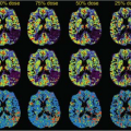
FIGURE 65.4. A middle-age man with hepatocellular carcinoma underwent free-breathing dynamic contrast-enhanced magnetic resonance imaging study and data obtained were analyzed using the distributed parameter model. Sagittal T1-weighted images obtained before (upper left) and after (upper right) contrast administration show position of the tumor (arrows) and the area from which parametric maps are calculated. The parametric maps of the tumor region demonstrating blood flow (F), hepatic perfusion index (α), hepatic arterial perfusion (F_A), portal venous perfusion (F_PV), contrast arrival time (t₀), mean transit time (t₁), fractional intravascular volume (v₁), fractional interstitial volume (v₂), extraction fraction (E), and permeability surface area product (PS) are as shown. Note the increased hepatic perfusion index (α), but decreased portal venous perfusion (F_PV) within the tumor. The tumor does not show high permeability surface area product (PS) and reveals moderate mean transit time (t₁). (Images courtesy of Dr. Boon Cher Goh, National University Hospital and Prof. Tong San Koh, National Cancer Centre, Singapore.)

For MRI, 0.1 to 0.2 mmol/kg of gadolinium contrast agent and normal saline flush is usually administered in a dynamic fashion with an MR-compatible power injector. The rate of administration should be rapid enough to ensure adequate first-pass bolus arterial concentration of the contrast agent. At the same time, however, injection rate should not be too fast so as not to miss the aortic peak enhancement with acquisition temporal windows from 3 to 5 seconds. Generally, injection rates of 3 to 5 mL/s are used (Table 65.1). The contrast agent is usually flushed with about 20 to 40 mL of normal saline, which should be injected at the same rate as the contrast agent.

Motion-Related Issues

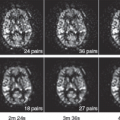
Respiratory motion is a major cause of image misregistration during a dynamic perfusion study of the liver, leading to errors in perfusion values and artifacts on parametric images.²⁴^,⁵⁵ Yet there has been no consensus as to whether the CT or MRI data should be acquired with suspended respiration or during shallow free-breathing (Fig. 65.4).²⁶^,⁵⁵^,⁶⁸ Suspended respiration is unlikely to be possible for perfusion studies lasting more than at least 45 to 60 seconds, which extend beyond the practical limit (approximately 30 seconds) for a single breath-hold in many patients. In MRI, image acquisition in sequential breath-hold is possible, whereby the entire liver volume is imaged twice during a period of 6 seconds’ breath-hold, followed by 6 seconds of breathing, and the entire cycle is repeated 40 times (Fig. 65.5). But this serial breath-hold approach requires more patient cooperation.⁷¹ If the patient is uncooperative, it may lead to motion artifacts because of the images being acquired during different
breath-hold conditions and over different image extents. Therefore, many investigators asked the patients to breathe quietly over a period of time, while they acquired CT or MR perfusion dataset. Consequently, soft tissue deformations occur because of respiratory and cardiac motion, requiring a motion correction step (Fig. 65.3). The specifics of liver perfusion imaging make this step particularly challenging for the following reasons. First, intensity values in the liver tissues and vessels can be locally and drastically changed by the contrast agent administration. Here, the specific challenge is that one aims to perform perfusion analysis on time-intensity curves on a per-pixel level when there is motion on the order of several pixels. Second, the geometric distortions of the liver are nonrigid and the degree of hepatic contour deformation during respiration can be large. Finally, the size and number of data volumes to register require a computationally efficient technique.⁷²

FIGURE 65.5. A 56-year-old man with metastatic neuroendocrine tumor to the liver. Hepatic arterial perfusion (HAP) map (left), hepatic perfusion index (HPI) map (middle), and unenhanced T1-weighted image of the liver (right) show multiple hypervascular metastases. Whole-liver coverage imaging of the liver was performed using a sequential breath-hold magnetic resonance acquisition technique in the coronal plane, with two liver volumes acquired during a 6-second breath-hold followed by 6 seconds of breathing. In this imaging section, note multiple liver metastases showing increased HAP associated with high HPI. Even small metastases less than 1 cm in diameter (arrows) can be seen to exhibit this behavior, thus facilitating their detection.

For CT perfusion, several nonrigid registration approaches have been proposed, including free-form deformation method, viscous fluid deformation model, and volume-preserving fluid registration method.⁷³^,⁷⁴^,⁷⁵ There have been a few studies with the liver CT perfusion data addressing the misalignment and motion correction of the liver. Regardless of the methods used, most investigators agreed that better accuracy, reproducibility, and inter- or intraobserver variation of perfusion parameters can be achieved with motion correction rather than without.²⁴^,⁶⁰ For example, Ng et al.²⁴ recently reported that absolute values and reproducibility of CT perfusion parameters were markedly influenced by motion, and the best overall reproducibility was obtained with motion correction using an automated registration method.

For MRI perfusion, various kinds of rigid, nonrigid, or combined registration algorithms have been proposed to eliminate errors from motion in successive time-varying images of DCE-MRI. They include sequential elastic registration, pharmacokinetic model-driven nonrigid registration, and progressive principal component registration.⁷⁶^,⁷⁷^,⁷⁸^,⁷⁹ Although there is no consensus on which method is the best, the application of registration schemes before pixel-by-pixel pharmacokinetic analysis of perfusion MRI improved the accuracy of perfusion parameter measurement, regardless of the algorithms applied.⁷⁹ Inclusion of the right hemidiaphragm in dynamic studies can provide a contrast-invariant boundary and facilitate motion correction.

Clinical Application of Liver Computed Tomography and Magnetic Resonance Perfusion

Since Miles et al.³² and Scharf et al.⁸⁰ first described the feasibility of liver CT and MR perfusion, respectively, there has been a gradual increase in clinical use of perfusion imaging in liver tumors. Published clinical applications of liver perfusion include early detection of tumors, lesion characterization (differentiation between benign and malignant tumors), disease prognostication based on tumor vascularity, and monitoring therapeutic effects of various treatment regimens, including antiangiogenic drugs. Studies reporting on these indications are summarized in Tables 65.2 and 65.3.

Alteration of Computed Tomography and Magnetic Resonance Perfusion Parameters in Liver Tumors

Initial reports have been focused on how the perfusion parameters change in the tumors of the liver. Early work by Dugdale and Miles,³³ Miles et al.³⁷ Miles and Kelley,⁸¹ and Blomley et al.³⁴ on CT perfusion of liver metastases have shown increased arterial perfusion in liver metastases,

which were confirmed by other investigators, regardless of the modality used (CT vs. MRI), pharmacokinetic methods used, and subjects included (Fig. 65.6). For CT, Leggett et al.³⁶ also reported increased arterial perfusion and a decrease in portal liver perfusion in patients with metastatic diseases (Fig. 65.6). Their results were well in line with a common belief that liver metastases can increasingly draw blood supply from the hepatic artery. Several researchers have also confirmed this observation on MR perfusion, using variable analysis models. Totman et al.³⁸ and Miyazaki et al.³⁹ used a maximum slope method and demonstrated significantly increased HPI and significantly reduced portal perfusion in patients with metastasis (Figs. 65.5 and 65.7). Koh et al.³⁰ also showed that the mean HPI of metastases was increased up to 46% to 76% compared with normal liver tissue in three patients with liver metastasis by applying a dual-input, dual-compartment model on MR perfusion. In their study, the total hepatic perfusion of metastasis was lower than that of the surrounding parenchyma, reflecting the hypovascular nature of the metastases.

Only gold members can continue reading. Log In or Register to continue