2 Physics and Instrumentation in Doppler and B-mode Ultrasonography
Sound Propagation in Tissue
Speed of Sound
Sound propagation speeds depend on the properties of the transmitting medium and not significantly on frequency or wave amplitude. As a general rule, gases, including air, exhibit the lowest sound speed; liquids have an intermediate speed; and firm solids such as glass have very high speeds of sound. Speeds of sound in common media and tissues are listed in Table 2-1. For soft tissues, the average speed of sound has been found to be 1540 m/sec.1 Most diagnostic ultrasound instruments are calibrated with the assumption that the sound beam propagates at this average speed. Slight variations exist in the speed of sound from one tissue to another, but as Table 2-1 indicates, speeds of sound in specific soft tissues deviate only slightly from the assumed average. Adipose tissues have sound speeds that are lower than the average, whereas muscle tissue exhibits a speed of sound that is slightly greater than 1540 m/sec.
TABLE 2-1 Speed of Sound for Biologic Tissue
| Tissue | Speed of Sound (m/sec) | Change from 1540 m/sec (%) |
|---|---|---|
| Fat | 1450 | −5.8 |
| Vitreous humor | 1520 | −1.3 |
| Liver | 1550 | +0.6 |
| Blood | 1570 | +1.9 |
| Muscle | 1580 | +2.6 |
| Lens of eye | 1620 | +5.2 |
From Wells PNT: Propagation of ultrasonic waves through tissues. In Fullerton G, Zagzebski J, editors: Medical physics of CT and ultrasound, New York, 1980, American Institute of Physics, p 381.
Frequency and Wavelength
The number of oscillations per second of the piezoelectric element in the transducer establishes the frequency of the ultrasound wave. Frequency is expressed in cycles per second, or hertz (Hz). Audible sounds are in the range of 30 Hz to 20 kHz. Ultrasound refers to any sound whose frequency is above the audible range (i.e., above 20 kHz). Diagnostic ultrasound applications use frequencies in the 1-MHz to 30-MHz (1 million to 30 million Hz) frequency range. Manufacturers of ultrasound equipment and clinical users strive to use as high a frequency as practical that still allows adequate visualization depth into tissue (see section on attenuation). Higher frequencies are associated with improved spatial detail, or better resolution.
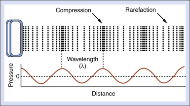
Figure 2-1 shows what might be called a snapshot of a sound wave, captured at an instant of time. It illustrates accompanying compressions and rarefactions in the medium that result from the particle oscillations. The wavelength λ is the distance over which a property of a wave repeats itself. It is defined by the equation
 (2-1)
(2-1)where c is the speed of sound and f is the frequency. Table 2-2 presents values for the wavelength in soft tissue, where the speed of sound is taken to be 1540 m/sec, for several frequencies. A good rule of thumb for tissues is the wavelength λt = 1.5 mm/F, where F is the frequency expressed in MHz. For example, if the frequency is 5 MHz, the wavelength in soft tissue is approximately 0.3 mm. Higher frequencies have shorter wavelengths and vice versa.
TABLE 2-2 Wavelengths for Various Ultrasound Frequencies
| Frequency (MHz) | Wavelength* (mm) |
|---|---|
| 1 | 1.54 |
| 2.25 | 0.68 |
| 5 | 0.31 |
| 10 | 0.15 |
| 15 | 0.103 |
* Assuming a speed of sound of 1540 m/sec.
Amplitude, Intensity, and Power
A sound wave is accompanied by pressure fluctuations in the medium. The pressure profile that could occur for the wave in Figure 2-1 might appear as in the graph in the lower part of this figure. The pressure amplitude is the maximal increase (or decrease) in the pressure caused by the sound wave. The unit for pressure is the pascal (Pa). Pulsed ultrasound scanners can produce peak pressure amplitudes of several million pascals in water when power controls on the machine are adjusted for maximal levels. As a benchmark for comparison, atmospheric pressure is approximately 0.1 MPa, so it is clear that ultrasound fields from medical devices significantly exceed this mark. The high-pressure amplitudes of an ultrasound pulse can easily burst contrast agent bubbles (see later) that are sometimes injected into the bloodstream to enhance echo signals. Diagnostic levels, however, are not believed to create biologic effects in tissues if such gas bodies are not present.
The intensity (I) of a sound wave at a point in the medium is estimated by squaring the pressure amplitude (P) and using I = P2/2ρc, where ρ is the density and c is the speed of sound. Units for ultrasound intensity are watts per meter squared (W/m2) or multiples thereof, such as mW/cm2. In water, a 2-MPa amplitude during the pulse corresponds to a pulse average intensity of 133 W/cm2! This is a high intensity, but, fortunately, it is not sustained by a diagnostic ultrasound device because the duty factor (i.e., the fraction of time the transducer actually emits ultrasound) typically is less than 0.005. Therefore, the time-averaged acoustic intensity from an ultrasound machine, found by averaging over a time that includes transmit pulses as well as the time between pulses, is much lower than the intensity during the pulse. Typical time-averaged intensities at the location in the ultrasound beam where the maximal values are found are on the order of 10 to 20 mW/cm2 for B-mode imaging. Doppler and color flow imaging modes have higher duty factors. Moreover, these modes tend to concentrate the acoustic energy into smaller areas. Time-averaged intensities for Doppler modes may be a few hundred mW/cm2 for color flow imaging and as high as 1000 to 2000 mW/cm2 for pulsed Doppler!2,3
Acoustic Output Labels on Machines
To help operators implement the ALARA principle, output labels are used that are related to the biologic effects of ultrasound.4 One of the potential effects is “cavitation,” which describes activity of small gas bodies under the action of an ultrasound field. When gas bodies are present, such as when there are contrast agents in the ultrasound field, cavitation increases the local stresses on tissue that are associated with the ultrasound waves. If the wave amplitude is high enough, collapse of the gas body occurs, and this is accompanied by localized energy depositions that significantly exceed depositions that might occur without cavitation. Cavitation is believed to be most closely associated with the peak negative pressure in the ultrasound wave. Scientists have developed a “mechanical index” (MI) that is derived from the peak negative pressure in the medium. For most ultrasound machines, the current maximum MI in the field is displayed in a prominent position on the display (Figure 2-2).
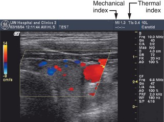
Another way that ultrasound energy may affect tissue is by heating through absorption of the waves. Absorption is one of the mechanisms that result in attenuation of a sound beam as it propagates through tissue. A corresponding index, the “thermal index” (TI) is displayed to indicate the likelihood of heating (see Figure 2-2). This is estimated using the time-averaged acoustic power or the time-averaged intensity, along with detailed mathematical models for the sound beam pattern and assumptions on the ultrasonic and thermal properties of the tissue. Depending on the application, a machine will exhibit either a soft tissue thermal index value (TIs) or a thermal index for the case in which absorbing bone is at the beam focus (TIb). TIc is a thermal index that is used for Transcranial Doppler studies because heating is likely to occur in the cranial bones.
The acoustic output labeling standard calls for a clear display of MI and TI.4 The standard is followed by most ultrasound equipment manufacturers, and it provides ultrasound system operators values of acoustic output quantities that are relevant to the possibility of biologic effects from the ultrasound exposures.
Decibel Notation
 (2-2)
(2-2)Thus, the decibel relation between two intensities is just the log of their ratio multiplied by 10. The same equation holds for expressing the ratio of two power levels. The difference in decibels between two powers is found by taking the log of their ratio and multiplying by 10.
Sometimes amplitudes rather than the intensities of two signals are used to express decibels. For a given decibel level, one must account for the fact that the intensity is proportional to the square of the amplitude. Substituting the corresponding amplitudes (A1 and A2) into Equation 2-2, squaring them, and taking into account that log (x2) is 2(log x), we have the relationship
 (2-3)
(2-3)Notice, the multiplicative factor is 20 rather than 10 when converting amplitude ratios to decibels.
Table 2-3 lists decibel values for various intensity and amplitude ratios. Notice that a 3-dB increase in the intensity is the same as doubling the quantity. A 10-dB increase corresponds to a 10-fold increase, and a 20-dB increase means that the intensity is multiplied by 100. The lower half of the table shows decibel changes corresponding to reductions of the intensity. A 3-dB decrease is the same as halving the intensity, and so forth.
TABLE 2-3 Decibel Differences Corresponding to Various Intensity and Amplitude Ratios*
| Amplitude Ratio (A1/A2) | Intensity Ratio (I1/I2) | Decibel Difference (dB) |
|---|---|---|
| 1 | 1 | 0 |
| 1.41 | 2 | +3 |
| 2 | 4 | +6 |
| 2.828 | 8 | +9 |
| 3.16 | 10 | +10 |
| 4.47 | 20 | +13 |
| 10 | 100 | +20 |
| 100 | 10,000 | +40 |
| 1 | 1 | 0 |
| 0.707 | 0.5 | −3 |
| 0.5 | 0.25 | −6 |
* For example, if I1 is 10 times I2, it is 10 dB greater than I2. A 20-dB difference between two signals corresponds to both a ratio of 10 for their amplitude or a ratio of 100 for their intensities, and so forth.
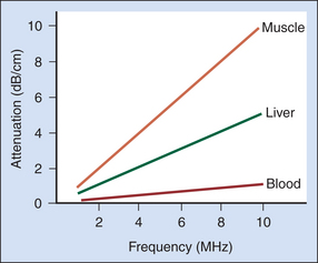
Attenuation
The rate of attenuation in relation to distance is called the attenuation coefficient, expressed in decibels per centimeter. The attenuation coefficient depends on both the medium and the ultrasound frequency. Figure 2-3 illustrates attenuation coefficients for a few tissues, plotted versus the frequency. Attenuation is quite high for muscle and skin, has an intermediate value for large organs such as the liver, and is very low for fluid-filled structures. For the liver, it is approximately 0.5 dB/cm at 1 MHz, whereas for blood, it is about 0.17 dB/cm at 1 MHz. An important characteristic of attenuation is its frequency dependence. For most soft tissues, the attenuation coefficient is nearly proportional to the frequency.1 The attenuation expressed in decibels would roughly double if the frequency were doubled. Thus, higher-frequency sound waves are more severely attenuated than lower-frequency waves, and the high-frequency beams cannot penetrate as far as low-frequency beams. Diagnostic studies with higher-frequency sound beams (7 MHz and above) are usually limited to superficial regions of the body. Lower frequencies (5 MHz and below) must be used for imaging large organs, such as the liver.
Reflection
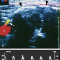
Figure 2-4 shows an ultrasound image of the carotid artery of a normal adult. The walls of the vessel can be seen because of reflection of sound waves. Echoes from muscle and other tissues are also produced by reflections and by ultrasonic scatter. Both reflection and scatter contribute to the detail seen on clinical ultrasound scans.
The reflection coefficient quantifies the relative amplitude of a wave reflected at an interface. It is the ratio of the reflected amplitude to the incident amplitude. For perpendicular incidence of the ultrasound beam on a large, flat interface (Figure 2-5), reflection coefficient (R) is given by
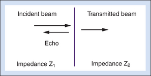
 (2-4)
(2-4)where the impedances Z1 and Z2 are identified in Figure 2-5.
Equation 2-4 shows that the larger the difference between impedances Z2 and Z1, the greater will be the amplitude of the echo from an interface, and hence, the less will be the transmitted signal. Large impedance differences are found at tissue-to-air and tissue-to-bone interfaces. In fact, such interfaces are nearly impenetrable to an ultrasound beam. In contrast, significantly weaker echoes originate at interfaces formed by two soft tissues because, generally, there is not a large difference in impedance between soft tissues.5
Large, smooth interfaces, such as those indicated in Figure 2-5, are called specular reflectors. The direction in which the reflected wave travels after striking a specular reflector is highly dependent on the orientation of the interface with respect to the sound beam. The wave is reflected back toward the source only when the incident beam is perpendicular or nearly perpendicular to the reflector. The amplitude of an echo detected from a specular reflector thus also depends on the orientation of the reflector with respect to the sound beam direction. The ultrasound image in Figure 2-4 was obtained using a linear array probe, which sends individual ultrasound beams into the scanned region in a vertical direction as viewed on the image. Sections of the vessel wall that are nearly horizontal yield the highest amplitude echoes and hence appear brightest because they were closest to being perpendicular to the ultrasound beams during imaging. Sections where the vessel is slightly inclined are seen as less bright.
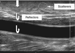
Scattering
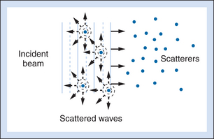
For interfaces whose dimensions are small, reflections are classified as “scattering.” Much of the background information viewed in Figure 2-4 results from scattered echoes, where no one interface can be identified but usually echoes from many small interfaces are picked up simultaneously. The scattered waves spread in all directions, as suggested in Figure 2-6. Consequently, there is little angular dependence on the strength of echoes detected from scatterers. Unlike the vessel wall, which is best visualized when the ultrasound beam is perpendicular to it, the scatterers are detected with relatively uniform average amplitude from all directions. Echoes resulting from scattering within organ parenchyma are clinically important because they provide much of the diagnostic detail seen on ultrasound scans.
In Doppler ultrasound, blood flow is detected by processing signals resulting from scattering by red blood cells. At diagnostic ultrasound frequencies, the size of a red blood cell is very small compared with the ultrasonic wavelength. Scatterers of this size range are called Rayleigh scatterers. The scattered intensity from a distribution of Rayleigh scatterers depends on several factors: (1) the dimensions of the scatterer, with a sharply increasing scattered intensity as the size increases; (2) the number of scatterers present in the beam (e.g., Shung has demonstrated that when the hematocrit is low, scattering from blood is proportional to the hematocrit6); (3) the extent to which the density or elastic properties of the scatterer differ from those of the surrounding material; and (4) the ultrasonic frequency. (For Rayleigh scatterers, the scattered intensity is proportional to the frequency to the fourth power.)
Nonlinear Propagation
A sound wave traveling through tissue will also undergo gradual distortion with distance if the amplitude is high enough. This is a manifestation of nonlinear sound propagation, and it leads to creation of harmonic waves, or waves that have frequencies that are multiples of that of the original transmitted wave. When partial reflection of the distorted beam occurs at an interface, the reflected echo consists of both the original, “fundamental frequency signals” and harmonic components. A 3-MHz fundamental echo is accompanied by a 6-MHz second harmonic echo and so on. Higher-order harmonics are possible, but attenuation in tissue usually limits the ability to detect them. Although the second harmonic echoes themselves are of lower amplitude than the fundamental, it is possible to distinguish them from the fundamental in the processor of an ultrasound machine and to use them to construct an image, called a tissue harmonic image.7
B-Mode Imaging
Range Equation
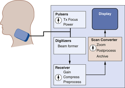
Ultrasound imaging is done using pulse-echo techniques. An ultrasonic transducer is placed in contact with the skin (Figure 2-7). The transducer repeatedly emits brief pulses of sound at a fixed rate, called the pulse repetition frequency, or PRF. After transmitting each pulse, the transducer waits for echoes from interfaces along the sound beam path. Echo signals picked up by the transducer are amplified and processed into a format suitable for display.
The distance to a reflector is determined from the arrival time of its echo. Thus,
 (2-5)
(2-5)where d is the depth of the interface, T is the echo arrival time, and c is the speed of sound in the tissue. The factor 2 accounts for the round-trip journey of the sound pulse and echo. Equation 2-5 is called the range equation in ultrasound imaging.8 A speed of sound of 1540 m/sec is assumed in most scanners when calculating and displaying reflector depths from echo arrival times. The corresponding echo arrival time is 13 µs/cm of the distance from the transducer to the reflector.
Signal Processing
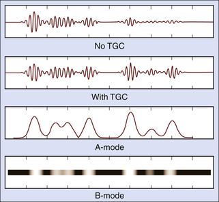
To create images, pulses of sound are transmitted along various beam lines, each followed by reception and processing of resultant echo signals. Imaging is done with transducer arrays, where echo signals are acquired by individual elements and are combined within a beam former into a single signal for each beam line. The role of the beam former will be discussed in more detail later. Following the beam former, echo signal processing for imaging consists of amplifying the signals; applying time gain compensation to offset effects of beam attenuation; applying nonlinear, logarithmic amplification to compress the wide range of echo signal amplitudes (called the displayed echo dynamic range) into a range that can be displayed effectively on a monitor; demodulation, which forms a single spike-like signal for each echo; and brightness-mode (B-mode) processing. The B-mode display is used in imaging. Signal processing steps are shown in Figure 2-8.
Forming the Image
Two well-known echo display techniques are also illustrated in the lower two panels of Figure 2-8. The amplitude-mode (A-mode) display is a presentation of the echo signal amplitude versus the echo return time, or the reflector depth. This is a one-dimensional display portraying echo signals and their amplitudes along a single beam line (i.e., along one direction). In contrast, the more versatile B-mode display is used for gray-scale imaging. The display is formed by converting echo signals to dots on a monitor, with the brightness indicating echo amplitudes.
In B-mode scanning, sound beams are swept over a region (Figure 2-9), and echo signals are registered on a two-dimensional (2D) matrix in a position that corresponds to their anatomic origin. Registration is done by placing the B-mode dots along a line that corresponds to the axis of the ultrasound beam as it sweeps across the scanned field; the proper depth of each echo is determined from the arrival time. In Figure 2-9, the sound beam is swept by electronic switching between groups of elements in a linear array transducer. The B-mode display on the monitor follows the axis of the ultrasound beam as it is swept across the imaged region. Usually, 100 to 200 or more separate ultrasound beam lines are used to construct each image. Most ultrasound systems have controls that allow the operator to vary the beam line density, either directly or indirectly when some other image-processing control is manipulated.
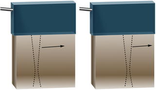
Image Memory
Image attributes such as the echo amplitude at each pixel location are represented using a sequence of 1s and 0s, as is the practice for digital devices. The fundamental unit of storage in a digital device is a singular entity called a bit. A single bit can take on a value of either 1 or 0, but by grouping bits into multibit storage cells, each multibit word can represent a large range of values because of the different combinations of 1 and 0 that can be accommodated. For example, “8-bit” memories divide the echo signal into 255 (28) different amplitude levels and store an appropriate level at each pixel location. Twelve-bit memories represent the echo amplitudes using 4096 (212) levels, and so forth. The more bits (amplitude levels), the more different shades of gray are possible from the stored image, especially during postprocessing (see later). Modern scanners also allow storage of cine loops, using a memory that can retain many separate images.
 (2-6)
(2-6) (2-7)
(2-7)Transducer Properties
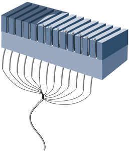
Internal components of an array transducer are shown in Figure 2-10. In the figure, the elements are seen from the side, and the ultrasound waves would be projected upward. The thickness of the piezoelectric element governs the resonance frequency of the transducer. Quarter-wave matching layers between the piezoelectric elements and a protective outer faceplate are used on most transducers. Analogous to special optical coatings on lenses and on picture frame glass, the matching layers improve sound transmission between the transducer and the patient. This improves the transducer’s sensitivity to weak echoes. Backing material is often used in pulse-echo applications to dampen the element vibrations after the transducer is excited with an electric impulse. Dampening shortens the duration of the transmitted pulse, improving the axial (or range) resolution. With optimized designs of the matching and backing layers, transducers can be made to operate over a range of frequencies. Hence, ultrasound machines provide a frequency control switch that the operator manipulates to select the frequency from a menu of choices available for each probe. Some transducers have sufficient frequency range that harmonic imaging can be done, where a low-frequency transmit pulse is sent out, and echoes whose frequency is twice that transmitted are detected and used in imaging.
Types of Transducers
The operation of three principal types of array transducers is presented in Figure 2-11
Related posts:
 Normal Cerebrovascular Anatomy and Collateral Pathways
 Controversies in Venous Ultrasound
 Nonimaging Physiologic Tests for Assessment of Lower Extremity Arterial Disease
 Ultrasound Assessment of the Abdominal Aorta
 Evaluation of Organ Transplants
Stay updated, free articles. Join our Telegram channel

Full access? Get Clinical Tree


