Diffusion is a powerful diagnostic tool that measures water molecule displacement of the size order of cell structures (a few micrometers). Hence it is sensitive to microstructural changes in brain tissue, even before these changes can be detected by other types of magnetic resonance imaging (MRI).
Water diffusion in the brain is relatively restricted, and, depending on the parameters of the diffusion pulse sequence, one can observe more or less of this restriction. The measured water diffusion coefficient depends on the (b values); thus the term apparent diffusion coefficient (ADC) is used.
Water diffusion in the brain is anisotropic, meaning that it is facilitated parallel to myelin fibers and axons and restricted perpendicular to them. The tensor model is adopted to describe this diffusion anisotropy, and it allows one to quantify anisotropy parameters (related to white matter integrity) and to reconstruct the trajectory of white matter fibers (diffusion tractography).
1.1 Introduction
Diffusion weighted images (DWIs) provide tissue contrast related to the thermally driven random motion (Brownian motion) of water molecules in brain tissue. Water diffusion is heavily restricted by the brain tissue microstructure, and this restriction is higher when it occurs perpendicular to the white matter fibers (diffusion anisotropy). This restriction to water diffusion has two important consequences: First, any changes at the cytoarchitecture level will be reflected in the DWI, making this method extremely sensitive to pathological changes; and second, based on the orientation of the faster diffusion in a voxel, white matter trajectories can be reproduced. This is the principle behind diffusion tractography.
1.2 Diffusion Weighted Imaging
1.2.1 Brownian Motion
Due to thermal energy, water molecules in a liquid state are in constant motion, following a random pathway where the direction of the motion changes with the collisions of water molecules. This type of motion is called brownian motion, named after the botanist Robert Brown, who first described it in 1827 after observing the motion of pollen suspended in water. In 1906 Albert Einstein described this motion mathematically, introducing the idea of random walk and the self-diffusion coefficient D. In this random walk (▶ Fig. 1.1) it is impossible to predict the distance that a given water molecule will diffuse in a given time, but it is possible to obtain a statistical value on how a whole group of water molecules will diffuse. This value is the mean square displacement <r2>, which reflects the mean of the gaussian distribution of displacements that water molecules accomplish in a given time period (see ▶ Fig. 1.1). As stated by the Einstein equation of diffusion in one dimension, <r2> increases with the diffusion time t (the observation time in the measurement), and the diffusion coefficient D is the proportionality constant, with a physical unit of mm2/s:
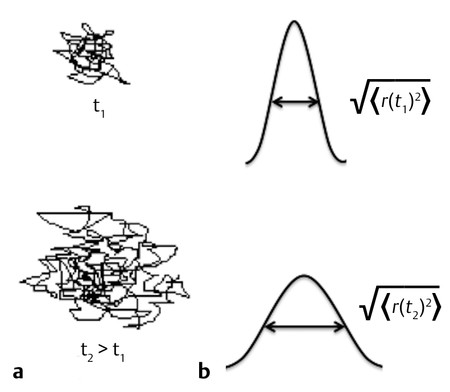
Fig. 1.1 (a) Example of random water molecule trajectories (“random walk”) during diffusion (brownian motion) and (b) gaussian distribution of water molecule displacements characterized by the root mean square displacement as a function of time.
 (1.1)
(1.1)
1.2.2 Stejskal and Tanner
In 1965 Stejskal and Tanner introduced the idea of measuring the diffusion coefficient of liquids by nuclear magnetic resonance (NMR) using pulsed gradients before and after the application of the 180-degree pulse in the spin-echo (SE) sequence (▶ Fig. 1.2). The first pulsed gradient causes a fast and controlled dephasing of the spins, afterward a 180-degree pulse is applied, which inverts all spins and initiates the process of spins rephasing for later formation of the echo. But, for the complete rephasing of the spins to occur, it is necessary to apply again exactly the same pulsed field gradient (with the same amplitude G and duration δ) that was applied before the 180-degree pulse, in order to compensate for the dephasing caused by the first pulsed gradient. If the spins do not change position relative to the applied field gradient during the time interval Δ, the time between the two pulsed field gradients, all spins will be correctly rephased and will contribute to the echo signal. However, most of the echo signal comes from water, which is in constant motion, and from the Einstein equation we know that, after a given time Δ the 〈r2〉 will be nonzero. Hence the location of the water molecules relative to the applied pulsed gradient will change, and as a consequence water diffusing spins will not be correctly rephased and will not contribute to the signal of the echo. By measuring the signal intensity of the SE with (S) and without (S0) the application of the pulsed field gradients the diffusion coefficient D can be calculated from the Stejskal and Tanner equation:
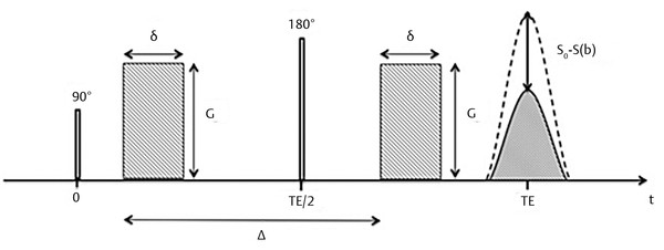
Fig. 1.2 Stejskal and Tanner pulse sequence for the measurement of diffusion. G, gradient amplitude; δ duration of the gradient pulse; Δ, interval between gradient pulses; TE, echo time. S0, signal without applying gradient pulses; S(b), signal after applying gradient pulses.
 (1.2)
(1.2)
where b is known as the b factor of the diffusion acquisition and depends on the pulse sequence parameters as shown in the next equation,
 (1.3)
(1.3)
with γ being the gyromagnetic ratio.
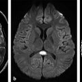
By increasing the b factor in the diffusion acquisition, more diffusion weight will be introduced in the images. When b = 0 (zero of diffusion weight) is applied, the result is basically a T2-weighted image, with high signal intensity for liquids (▶ Fig. 1.3a). When b = 1,000 s/mm2 is applied we obtain a DWI, where higher diffusion is denoted by hypointensity (strong signal attenuation), and slower diffusion (restriction to diffusion) is denoted by high signal intensity (▶ Fig. 1.3b).
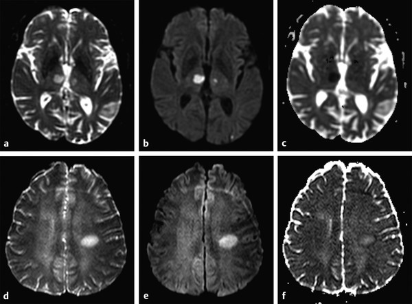
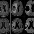
Fig. 1.3 (a) Non–diffusion weighted imaging (DWI) (b = 0 s/mm2) of a stroke patient presenting two thalamic lesions. (b) DWI (b = 1,000 s/mm2) with high signal intensity in both lesions. (c) Corresponding apparent diffusion coefficient (ADC) map confirming the restriction to diffusion in the lesions with a decrease in ADC. (d) Non-DWI (b = 0 s/mm2) of another stroke patient with a left subacute lesion. (e) DWI (b = 1,000 s/mm2) presenting high signal intensity in the lesion (T2 shine-through effect). (f) Corresponding ADC map showing that there is no restriction of diffusion, but rather an ADC increase in the lesion.
1.2.3 T2 Shine-through Effect and Apparent Diffusion Coefficcient Map
The interpretation of signal intensity in the DWI is not always straightforward. Sometimes the signal intensity may be high in both the non-DWI (b = 0) and the DWI (b > 0), independent of restriction to diffusion (▶ Fig. 1.3d,e). This is because DWIs are inherently also T2-weighted images because they are acquired with relatively long echo times (TEs) and long repetition times. In this case, the high signal intensity in the DWI may be due only to the T2 shine-through effect. To elucidate this question it is suggested to calculate the actual D for each voxel in the image as follows:
 (1.4)
(1.4)
where Sb1 and Sb2 are the signal intensities obtained with two different b values and b1 < b2. If we solve this equation for each voxel in the image, we obtain the so-called apparent diffusion coefficient (ADC) map (▶ Fig. 1.3c,f). In the ADC map, signal intensity directly reflects the ADC value, which is highest where there is free diffusion, like in the ventricular cerebrospinal fluid (CSF) with an ADC ≈ 3.2 × 10⁻³ mm2/s, and lowest in regions of restricted diffusion, i.e. in the white matter with an ADC ≈ 0.7 × 10⁻³ mm2/s. It is important to observe that, as indicated by the name of apparent diffusion coefficient, the calculated ADC in brain tissues depends on the choice of b1 and b2. Conventionally, in the brain the two b values chosen are 0 and 1,000 s/mm2, but different values can also be used. It is also possible to acquire images with more than two b values to obtain a better approximation of the ADC. In this case, the obtained signal intensity is fitted to an exponential function of b, derived from Equation ▶ 1.2:
 (1.5)
(1.5)
However, it has been shown that, for calculation of the ADC, it is not efficient in terms of signal to noise ratio (SNR) to use more than two b values. Two b values are enough, and, ideally, for in vivo brain measurements the difference between them should be approximately 1,000 to 1,500 s/mm2.1
1.2.4 Restriction of Water Diffusion in Brain Tissue
ADC as a Marker of Tissue Microstructure
Diffusion of water in biological tissues and in the brain is strongly restricted; water molecules constantly encounter barriers (e.g., cell membranes, myelin fibers, and axonal projections), which prevent the water from diffusing freely, such as it would in a glass of water. The water root mean square displacements that occur in the brain within the diffusion times used in conventional DWI are on the order of a few micrometers, which corresponds to the order of the size of cell structures. Hence the ADC measured in brain tissues reflects water motion restricted by these cell structures and is thus an extremely sensitive marker of tissue microstructure. For instance, it is possible to detect restriction in diffusion (decreased ADC) when there is an increase in cellular density caused by tumor growth or with cellular swelling in cytotoxic edema. On the other hand, the increase of extracellular space caused by vasogenic edema, demyelination, or axonal loss, results in an increase of the observed ADC. Any biological or pathological change that causes changes in the tissue microstructure will be in principle detected by changes in the ADC, which renders the DWI technique very powerful.
Size of Tissue Compartments
The size of the tissue compartments where water can diffuse plays an important role in the resulting ADC. Within one compartment water may diffuse freely, but if the diffusion time Δ of the experiment is long enough for the water molecules to reach the limits of the compartment, the chance that the water molecules will bounce back to the center of the compartment is greatly increased. As Δ increases, more water molecules will hit “the walls” of the compartment, and the observed <r2> will be smaller than that expected for free diffusion as illustrated in (▶ Fig. 1.4). Because of this effect it is advisable to keep a constant Δ value unless the intention is to determine the size of tissue compartments.2
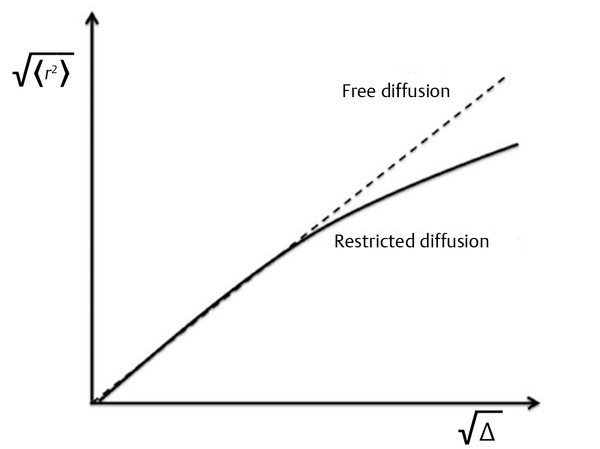
Fig. 1.4 Mean square displacement as a function of diffusion time showing the effect of restriction.
Influence of the b Factor on the ADC
As described in Equation ▶ 1.3 the b factor depends on the characteristics of the applied pulsed field gradients and on the diffusion time Δ. For the reasons already explained it is recommended to maintain Δ as a fixed value and to increase the b value only by increasing the diffusion gradient field strength (G). The stronger the applied pulsed field gradients, the higher the capacity of the gradients to cause dephasing, and signal attenuation will be measured even in the presence of very slow diffusion. This means that the higher the b value, the higher the contribution of the slow diffusing compartments will be in the final DWI. As the b value increases (> 1,000 s/mm2) the resulting ADC becomes smaller.3 This is because the obtained ADC in brain tissues is the average of the diffusion of several tissue compartments in the voxel, and as the b value increases and diffusion rate decreases, the contribution of slow diffusion compartments becomes higher. If signal intensity is plotted on a logarithmic scale as a function of b, the signal intensity decreases almost linearly until a value of 1,000 s/mm2 is reached, but above 1,000 s/mm2, the slope of the signal attenuation begins to change (▶ Fig. 1.5). For this reason, when using high b values (> 1,000 s/mm2) the signal attenuation is better described with a biexponential model.3 This biexponential behavior will be encountered only for voxels where compartments with different diffusions coexist, as in the white matter, whereas in the CSF within the ventricles signal attenuation will be monoexponential. By measuring the DWI signal as a function of different b values up to 4,000 to 6,000 s/mm2 Clark and Le Bihan3 estimated the fast diffusing fraction in brain tissue to be ~ 0.7, too large to be reflecting only the diffusion in the extracellular space, as discussed in their study.
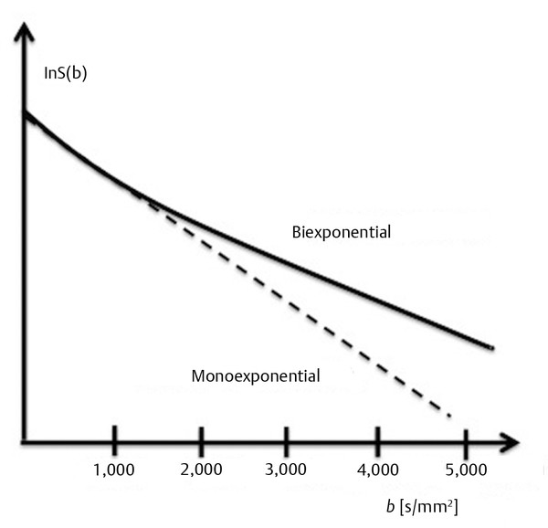
Fig. 1.5 Nonlinearity of diffusion in white matter at high b values.
Choice of the b Value
The question now arises as to how high the chosen b value should be. The slower the diffusion in the tissue, the higher the b value needs to be; on the other hand, if the b value is too high, the resulting DWI is very noisy. A b value of ~ 1/ADC of the tissue of interest is suggested to be optimal, but given that the TE needs to be increased with higher b values (due to the use of stronger gradients), and that a longer TE leads to a lower SNR, the optimal b becomes ~ 0.9/ADC.4,5 For brain studies a b value of 1,000 s/mm2 is commonly used and results in an effective compromise between diffusion sensitivity and SNR. Nevertheless, for lesions with a stronger restriction to diffusion than that in normal white matter (i.e., in tumors), it is interesting to use higher b values (i.e. b = 2,000 s/mm2) to increase the sensitivity of the method.6,7,8 Hence the ability to obtain a valuable DWI will be strongly related to the strength of the gradient coils and the maximum b values that can be achieved.
1.2.5 Anisotropy of Water Diffusion in the Brain
Isotropic and Anisotropic Diffusion
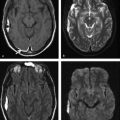
Sometimes the barriers that restrict water diffusion in brain tissues are isotropically distributed (▶ Fig. 1.6a), which means that diffusion will be restricted equally in all directions. At other times these barriers will be distributed anisotropically, resulting in stronger diffusion restrictions perpendicular to the barriers (▶ Fig. 1.6b). In white matter water, diffusion is facilitated parallel to axonal projections and myelin fibers, and it is restricted perpendicular to them. Thus the measured ADC depends on the direction of the applied pulsed field gradient. This is clearly illustrated in ▶ Fig. 1.7a–c, where one can observe the DWI with the diffusion gradients applied in the three orthogonal directions. When these images are compared important differences are visible, in particular in the region of the splenium of the corpus callosum, where there is high signal intensity for the image acquired with diffusion gradients applied in the z direction, indicating restriction to diffusion in the inferior–superior orientation, and very low signal intensity when the diffusion gradient is applied in the x direction, indicating unhindered diffusion in the right-to-left orientation, parallel to the corpus callosum fibers. This region in the brain is known to have the highest values of diffusion anisotropy. The term anisotropy indicates that water diffusion in brain tissue depends on orientation. To obtain DWI results that are independent on orientation, one needs to calculate the average of the three DWIs obtained with the pulsed diffusion gradients applied in the three orthogonal directions (▶ Fig. 1.7a–c). This average image is known as the isotropic DWI and is used to calculate the ADC (▶ Fig. 1.7d).
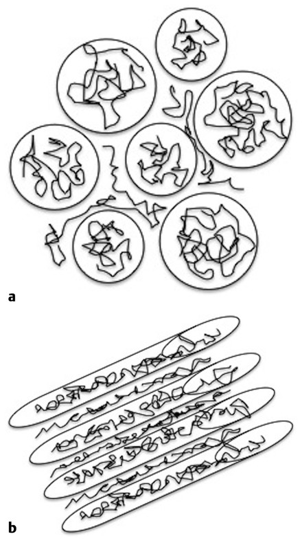
Fig. 1.6 (a) Isotropic and (b) anisotropic display of the barriers to diffusion.
Related posts:
 Diffusion Weighted Imaging in the Evaluation of Brain Tumors
 Diffusion Weighted Imaging in Hemorrhage
 Diffusion Weighted and Diffusion Tensor Imaging in Aging
 Diffusion Weighted Imaging and Diffusion Tensor Imaging in Demyelination and Toxic Diseases
 Diffusion Weighted Imaging and Diffusion Tensor Imaging in Head and Neck Diseases
 Diffusion Weighted and Diffusion Tensor Imaging in Infectious Diseases
Stay updated, free articles. Join our Telegram channel

Full access? Get Clinical Tree


