Radionuclides
Half-life
Mode of decay (%)
E β + max(MeV)
11C
20.4 min
β + (100)
0.970
13N
10 min
β + (100)
1.2
15O
2 min
β + (100)
1.74
18F
110 min
β + (97)
0.64
EC (3)
68Ga
68 min
β + (89)
1.90
EC(11)
82Rb
75 s
β + (95)
3.15
EC(5)
124I
4.2 d
β + (23)
2.14
EC(77)
Detectors in PET Scanners
Several types of scintillation detectors are available for PET scanners and their properties are illustrated in Table 8.1. NaI(Tl) was initially used in earlier PET scanners, but nowadays commercial manufacturers mostly use BGO, LYSO and LSO detectors because of their favorable characteristics in pulse production. All three detector materials are not hygroscopic obviating the need for hermetic sealing. They all have high stopping power (high density and linear attenuation coefficient), but LSO and LYSO have shorter scintillation decay time (40 ns and 50 ns, respectively) than BGO (300 ns) and have higher light output (30 photons and 25 photons vs. 6 photons). However, due to the intrinsic property, the energy resolution of these detectors is poor. It is to be noted that LSO and LYSO contain a naturally occurring radioisotope of its own, 176Lu, with an abundance of 2.6 % and a half-life of 3.8 × 10⁸ years. This radionuclide decays by emission of β − rays and x-rays of 88–400 keV. However, the activity level is low enough to ignore radiation exposure from 176Lu, and its photon energy lower than 511 keV does not cause a major problem in PET imaging.
GSO has been used in PET scanners by some manufacturers, despite its lower light output and stopping power than LSO. These crystals are fragile and require great care in fabrication.
BaF2 has the shortest decay time of 0.6 ns and is primarily used in time-of-flight PET scanners that are rarely used clinically.
Semiconductors such as lithium-activated germanium and silicon (Ge(Li) and Si(Li)) detectors are used for photon detection. Photons eject an electron from the atomic orbital following an interaction with these materials and create a positively charged hole in the atom. The electron-hole pair moves as current, when a high voltage is applied. These are called photodiodes and do not require any PM tube for amplification of pulses. High voltage application causes some electron multiplication in the detector, but in the absence of PM tubes, a large electron multiplication does not occur. The output signal is therefore weaker than the conventional PM tube signal resulting in poorer detection efficiency and so they are not used in PET scanners . A separate category of semiconductor detectors are cadmium-zinc-tellurium (CZT) or cadmium-tellurium (CdTe) that have relatively high atomic numbers (high stopping power) and excellent energy resolution (~ 5 %). Currently, the CZT detector has been used in commercial PET scanners offering high resolution and low noise images and promising a great potential for future use.
PM Tubes and Pulse-Height Analyzers
Like conventional cameras, PET scanners use PM tubes and pulse-height analyzers (PHA) for determining the locations of the origin of pulses and their amplitudes. As mentioned in Chap. 8, PM tubes convert light photons arising from the interaction of γ-rays in detectors to pulses, which are used to determine the X-, Y-positions of the two detectors that detect the two 511-keV photons (discussed later), and the PHA is used to check if the pulse height is within the acceptable range, which is normally set at 350 to 650 keV for 511-keV annihilation photopeak in PET scanners.
PET Scanners
In original PET scanners, many detectors (hundreds to thousands), each connected to a photomultiplier tube , are arranged in multiple circular, hexagonal, or orthogonal rings. The number of rings in PET scanners , and the number of crystals per ring vary with the manufacturer. The number of rings and, hence, the width of the array of rings define the axial field of view. Despite the advantage of good resolution with these scanners, the use of many PM tubes and packing them with as many detectors is very costly and impractical. To circumvent this problem, blocks of detectors connected to fewer PM tubes have been designed, which are described below.
Block Detectors
In modern PET scanners , the block detector is used, in which small detectors are created by making partial cuts on the front surface of a block of detector crystal and each block detector is coupled on the back side to 2–4 PM tubes. A schematic block detector is shown in Fig. 13.1. Typically, each block is about 3 cm deep and grooved into 6 × 8, 7 × 8, or 8 × 8 elements by partial cuts through the crystal with a saw. Each element is considered a small detector. The cuts are made at varying depths, with the deepest cut at the edge of the block. The cuts are filled with opaque reflective materials to prevent spillover of light between elements. The size of each detector varies from 3 to 6.5 mm and is one of the important parameters that determine the spatial resolution.
Fig. 13.1
A schematic block detector is segmented into 8 × 8 elements, and four PM tubes are coupled to the block for pulse formation. The pulses from the four PM tubes (A, B, C, and D signals) determine the location of the element in which 511-keV γ-ray interaction occurs, and the sum of the four pulses determines if it falls within the energy window of 511 keV
The block detectors are arranged in an array of full or partial rings with a diameter of 80–90 cm. The full ring array may be in the form of a circular or hexagonal shape. Two configurations of block detectors adopted by several manufacturers are shown in Fig. 13.2. Siemens mCT has 32,448 crystals arranged in 192 block detectors with four PM tubes per block, whereas in Philips Healthcare’s Gemini TF Big Bore scanner, 28,336 crystals coupled to 420 PM tubes are arrayed in 28 pixelar modules.
Fig. 13.2
Two configurations of PET scanners. a A circular full ring scanner. b A hexagonal array of quadrant-sharing panel detectors
Coincidence Timing Window
In ideal coincidence counting in PET , the two 511-keV annihilation photons should be detected by the two detectors exactly at the same time. In reality, however, one photon may arrive at one detector earlier than the other in the opposite detector. This uncertainty in detection time is called the timing resolution or coincidence timing window. The timing resolution results from the difference in pulse formation in the detector primarily due to statistical variations in gain and scintillation decay time of the detector. Furthermore, there is a time delay in the arrival of one photon relative to the other, because of the difference in distances traveled by the two photons, particularly if the annihilation occurs at the edge of the FOV. This also adds to the timing resolution. For a whole-body scanner with a diameter of 1 m, the maximum distance traveled by one photon can be as large as 1 m, and the other photon travels almost no distance, if the annihilation occurs at the edge of the FOV. Because the velocity of light is 3 × 10⁸ m/s, the difference in the arrival times of the two photons is about 3–4 ns (time to travel 1 m). This is the limit of timing resolution of a PET scanner with 1-m diameter.
After annihilation, two timing signals A and B are formed with timing width, say τ, depending on the scanner system. Signal B may arrive at one detector just τ ahead of (Fig. 13.3a) or τ behind (Fig. 13.3b) the arrival of signal A, and both signals will be counted in coincidence. This is the extreme limit, and all other annihilation events overlapping in their time widths (Fig. 13.3c) will be counted as coincident events. Thus the timing resolution or coincidence timing window has to be a minimum of 2τ. The typical coincidence timing window of conventional PET scanners is set at 6–20 ns .
Fig. 13.3
Two time signals with time width τ define the coincidence timing window of 2τ. a Pulse 2 (dashed line) of time width τ arrives at the opposite detector just after the arrival of Pulse 1 (solid line) of time width τ at one of the detector pair, overlapping only at the edge and two events are counted in coincidence. b Pulse 2 of time width τ arrives at one of the detector pair exactly prior to the arrival of Pulse 1 of time width τ at the other detector, overlapping only at the edge and two events are counted in coincidence. c Pulse 2 overlaps Pulse 1 partially or completely depending on the time of arrival of the pulses at the detector pair, and two events are counted in coincidence. Both A and B indicate that the timing window of the coincidence circuit must be at least 2τ to detect all events in coincidence
In a PET scanner, each detector element is connected by a coincidence circuit with a time window to a set of opposite detector elements (both in plane and axial) . The number of opposite detectors can vary from one to a maximum of half the total number of detectors present in a ring. Each detector element can be connected in coincidence to a maximum of half the total number N of opposite detector elements (N/2). Note that less than N/2 detectors can also be connected. As shown in Fig. 13.4, depending on the number of opposite detectors connected, each detector element has a number of projections that define an angle of acceptance . These angles of acceptance for all detector elements in the ring form the transaxial FOV. The angle of acceptance increases with the number of opposite detector elements connected in coincidence and, hence, the FOV.
Fig. 13.4
The transverse field of view determined by the acceptance angles of individual detectors in a PET scanner. Each detector is connected in coincidence with as many as half the total number of detectors in a ring and the data for each detector are acquired in a “fan beam” projection. All possible fan beam acquisitions are made for all detectors, which define the FOV as shown in the figure. (Reprinted with the permission of the Cleveland Clinic Foundation.)
PET/CT Scanners
Parallel to SPECT/CT systems, PET/CT has been developed, in which functional PET images are fused with anatomical CT images to provide more accurate diagnosis of human diseases . In a PET/CT unit, both scanners are mounted on a common gantry with the CT unit in the front and PET unit in the back attached to the CT unit (Fig. 13.5). Typically, this is opposite to the SPECT/CT arrangement in which the SPECT camera is placed in the front and the CT unit in the back. Both units use the same scanning table. As in SPECT/CT, the centers of the PET FOV and CT FOV are separated by a fixed distance, called the displacement distance. The horizontal travel range of the scanning table varies with the designs of the scanners. The actual scan field is the maximum travel range of the scanning table minus the displacement distance. Typically, a CT scan is taken first of the patient on the scanning table and in the CT scan field. The table with the patient in the same position is moved to the PET scan field and imaging is performed. Note that 18F-FDG is administered 60–90 min prior to scanning, and low-intensity 511-keV photons in the patient do not interfere with the CT scan, because of the high intensity of the CT x-ray beam. Fusion of the two sets of images is performed by using commercial software as discussed under SPECT/CT . As described later, CT transmission data are used to calculate the attenuation factors for the PET emission data. The principle of attenuation correction is the same as described in SPECT/CT, based on the ratios of pixel data of a blank and the patient’s CT transmission scans. Factors affecting the attenuation corrections are discussed later.
Fig. 13.5
Schematic design of a PET/CT scanner
Because the position of the patient on the table does not change, both CT anatomical and PET functional images can be fused with accurate alignment providing better accuracy in detection of diseases. The overall accuracy of diagnosis increases by 20–25 % with PET/CT compared to either modality alone. Because CT scanning is fast, the total scanning time is significantly reduced, and the patient throughput is increased. Because of the increased reimbursement, whole-body imaging with PET/CT for accurate diagnosis of various cancers has become the standard of practice. The sale of PET/CT units worldwide has outpaced that of PET scanners with the sale of the latter dwindling.
Three manufacturers dominate the PET/CT markets: Siemens Healthcare, GE Healthcare, and Philips Healthcare. Each company has introduced several models in the market, making many technical improvements over the years. Current available PET/CT cameras have highly sophisticated features affording good quality images. The physical features of three PET/CT scanners from three manufacturers are listed in Table 13.2 and a commercial PET/CT scanner is shown in Fig. 13.6.
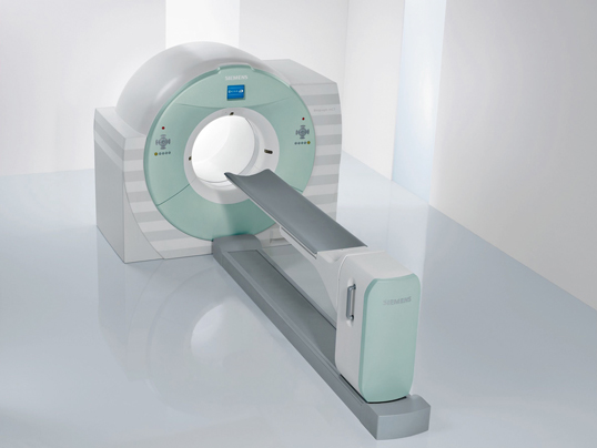
Fig. 13.6
A PET/CT scanner, Biograph mCT. (Image/Photo courtesy of Siemens Medical Solutions USA, Inc., Malvern, PA.)
Table 13.2.
Some features of commercial PET/CT scannersa
Model/product name | GE healthcare | Philips healthcare | Siemens healthcare |
|---|---|---|---|
Discovery PET/CT 710 | Gemini TF Big Bore (PET/CT) | Biograph mCT | |
Gantry dimensions, H × W × D, cm | 192 × 226.1 × 140 | 219 × 239 × 223.7 | 204 × 234 × 136 |
Weight, kg (lb) | 4,916 | 4,007 | 3,980 with TrueV |
Patient port (cm) | 70 | 85 | 78 |
Transmission source | CT attenuation correction | CT | CT |
Vertical travel, cm | 2.5–20.5 below isocenter | 40 | 53–96 |
Acquisition modes | 3-D, 4-D | 3-D, 4-D TOF | |
Horizontal speed | 100 mm/sec | 185 mm/sec | 0–200 mm/sec |
Number of detectors | 24 | 28 pixelar modules | 192 with TrueV |
Number of image planes | 47 | 45 or 90 | 109 with TrueV |
Number of crystals | 13,824 | 28,336 | 32,448 with TrueV |
Number of PMTs | 1,024 (256 quad-anode) | 420 | 4/block |
Physical axial FOV, cm | 15.7 | 18 | 21.6 with TrueV |
Detector material | LBSb | LYSO | LSO |
Crystal size, mm | 4.2 × 6.3 × 25 | 4 × 4 × 22 | 4 × 4 × 20 |
System sensitivity—3-D, kcps/uCi/cc/LLD (NEMA 2001) | 7 cps/KBq | 6,700 cps/MBq @ 10 cm > 18,000 with TOF | 9.5/435 keV with TrueV |
Transverse resolution @ 1 cm mm (NEMA 2001) | 4.9 VUE | 4.7 | 4.4 |
Axial resolution @ 1 cm mm (NEMA 2001) | 5.6 VUE | 4.7 | 4.5 |
Peak noise equivalent count rate, kcps (NEMA 2001) 3D | 130 @ 29.5 kBq/ml | 90 @ 14 kBq/ml (240 with TOF) | 175 @ 28 kBq/ml |
Scatter fraction—3-D (NEMA 2001) | 37 % | 26% | < 34 % |
Type of CT detector | Volara XT Digital DAS | Solid State—GOS | UltraFast Ceramic |
kV-range/mA-range | 700 or 800 mA | 90–140 kVp/20–500 mA | 80–140 kV/20–800 mA |
CTDI (dose/100 mAs) B/16 cm phant | Axial head: 18 mGy Axial body: 8 mGy | 10.17 mGy/100 mAs | 40/64 slice 9.3 mGy 128 slice 8.5 mGy |
Standard HC resolution (2 % MTF) | 17.1 lp/cm | 12 lp/cm | 16.4 lp/cm |
Number of slices | 16, 64, 128 | 16 | 40, 64 or 128 |
Reconstruction time: std/high res/topo | 16 FPS/35 FPS | Up to 20 images per sec | Up to 40 images per sec |
PET/MR Scanners
On the heels of success with PET/CT in clinical imaging, interest has grown considerably for similar application of PET/MR as a clinical diagnostic modality . MR provides anatomic and structural images with submillimeter spatial resolution offering a better soft-tissue contrast than CT. MR also has the great advantage of using magnetic radiofrequency, thus eliminating the radiation dose to the patient. The following is a brief description of currently available PET/MR scanners .
Principles of MR Imaging
It is beyond the scope of this book to describe in detail the principles of magnetic resonance (MR) imaging and the readers are referred to specific textbooks on MR imaging. The following is a brief summary of the subject.
MRI is based on the magnetic property of atomic nuclei . Protons and neutrons have magnetic moments due to inherent angular momentum and spin haphazardly (Fig. 13.7a). Nuclei containing even numbers of protons and neutrons possess no net magnetic moment, because of the cancellation of the individual magnetic moments by the even number of nucleons . Nuclei containing odd number of protons or neutrons, however, possess a net magnetic moment that has both a magnitude and a direction and behave like magnets. When these nuclei (or spins, as they are commonly called) are placed in a large external magnetic field (B0), they align themselves (at a slight angle) in either parallel or antiparallel direction to the magnetic field and also precess (rotate) at a frequency proportional to the strength of the field (Fig. 13.7b). The parallel spins remain in the lower energy state and the antiparallel ones in the high energy state, the energy difference being ΔE. Normally a slightly greater number of spins exist in parallel direction and they increase with the increase in magnetic field strength. These excess spins result in a net magnetization (Mz) with a measurable magnetic moment parallel to the field of B0 and they are said to be at equilibrium in the Z direction. If a radiofrequency pulse (RF), which is an oscillating electromagnetic field normally termed B1, is applied perpendicular to B0 at the precessional (resonant) frequency of the nuclei, the latter absorb energy from the RF field and make a transition to the high energy state. As a result, the longitudinal magnetization (Mz) flips towards the transverse plane (X–Y plane) at different angles depending on the strength of the RF pulse, thus causing transverse magnetization (Mxy). RF pulses that cause 90° flipping are called 90° pulses and produce maximum possible transverse magnetization (Fig. 13.8) and are commonly used in MR imaging. If a 180° pulse is applied, it will invert Mz to − Mz i.e. the longitudinal magnetization will be inverted in the opposite direction (Fig. 13.8).
Fig. 13.7
a Free protons spin randomly and their magnetic moments cancel each other, with a residual momentum due to an unpaired proton, if any. b When an external magnetic field, B0, is applied, the protons orient themselves in either parallel or antiparallel direction to the field B0. The number of parallel protons are slightly larger than antiparallel ones, thus creating a net magnetic moment in the direction of B0. The energy difference between the two groups is ΔE
Fig. 13.8
When a radiofrequency pulse (RF), B1, is applied to the MZ (longitudinal magnetization) in the presence of B0, MZ flips towards the transverse plane (X–Y) plane at different angles depending on the strength of B1. RF pulse that causes 90° flipping produces maximum transverse magnetization Mxy. If a 180° pulse is used, + MZ becomes − MZ
Hydrogen atoms have one proton in the nucleus and are abundant in the living body mostly in the form of water (70 %), with the remainder in tissues and fat. When a patient is placed in a magnetic field (B0) as in a MR machine, the tissues become magnetized due to excess parallel protons or spins that align with B0 and remain at equilibrium. When an RF pulse (commonly 90° pulse) is applied perpendicular to B0, the equilibrium of longitudinal magnetization is perturbed as a result of energy absorption from the RF field by the excess parallel spins of the nuclei, and the magnetization vector orients to the transverse or X–Y plane (at 90°for the 90° pulse). All nuclei remain in phase coherence, meaning magnetization vectors of all neighboring nuclei point to the same direction with maximum magnetization. If a receiver coil is placed perpendicular to the external field B0, the transverse magnetization (maximum Mxy) induces a current or a sinusoidal MR signal in the receiver coil according to Faraday’s law of induction. This signal is called free induction decay (FID) signal and its size increases with the strength of the magnetic field B0 and the magnitude of the RF pulse (B1). As the RF field is switched off, the FID signal decays resulting in the return of all nuclei to the original state they had before. This return is called relaxation of the nuclei. Two types of basic relaxation occur in tissues simultaneously, T1 and T2, and both contribute to the decay of the MR signal.
In T1 relaxation , nuclei give off their excess energy by spin-lattice interaction to the surrounding molecular structures (lattice) and start to regrow magnetization along B0, finally reaching the original value of maximum longitudinal magnetization at equilibrium. The rate of this regrowth is characterized by a tissue relaxation parameter called T1, which is defined by the time to recover 63 % of the maximum longitudinal magnetization following a 90° pulse (Fig. 13.9). T1 values depend on the vibrational frequencies and hence the physical characteristics of the molecules such as solid or liquid states, or stationary or moving structures.
In T2 relaxation following the shut-off of the RF pulse, all nuclei lose their phase coherence over time due to the random collision among neighboring nuclei (spin-spin interaction) thus losing energy to return to the original state of random phase. Random collision is caused by varying precessions of the nuclei at different velocities because of the small inhomogeneities of the magnetic field intrinsic to the structure of the tissues and also of the external field B0. The dephasing results in a fast exponential decay of the MR signal characterized by the time T2, which is given by the time interval between peak transverse signal and 37 % of the peak (1/e) (Fig. 13.10).
Fig. 13.9
Following a 90° RF pulse, longitudinal magnetization MZ is converted to zero at X–Y plane, but returns to equilibrium exponentially. It occurs through spin-lattice interaction with a relaxation constant T1, which is the time when 63 % of MZ is recovered
Fig. 13.10
Following a 90° RF pulse, MZ flips to X–Y plane (Mxy), which loses phase coherence due to spin-spin interaction in tissues and inhomogeneity of the external field. The FID signal decays exponentially with a time constant T2, during which the signal decays to 37 %
T1 values increase with higher magnetic field and are normally much longer than T2 values for most tissues. Both T1 and T2 values depend on the composition of tissues. For example, fat has a short T1 and fluid (cerebrospinal fluid, cyst, etc.) has longer T1, so fat is seen as bright, whereas fluid appears as dark. Other tissues fall within the range between the two. On the other hand, mobile molecules such as blood exhibit a long T2, whereas nonmoving structures like bone have a short T2.
MR signals depend on proton density, T1 and T2 relaxation time constants of different tissues in the body. One can obtain sufficient contrast between tissues by manipulating the timing, order, polarity and repetition frequency of RF pulses and B0. Tailoring of these parameters is alluded to as pulse sequence, the application of which depends on the type of tissue being imaged. Three major types of pulse sequences are spin echo (SE), inversion recovery (IR) and gradient recalled echo (GRE), the details of which are available in standard physics books. In spin echo pulse sequence, a 90° pulse is applied to cause transverse magnetization in tissues, followed by a 180° pulse to reverse it to the longitudinal magnetization. When all spins are rephased, an RF “echo” (a measureable MR signal) is produced and the time between the 90° pulse and the peak of the echo is called the time of echo (TE). The time between two successive 90° pulses is called the repetition time (TR). A spin-echo sequence of a short TR (e.g., 250–1000 ms) and a short TE (less than 25 ms) highlights the T1 difference in tissues and is called T1-weighting, whereas a combination of a long TR (2500–6500 ms) and a long TE (more than 75 ms) emphasizes T2 differences in tissues and hence the T2-weighting. In an IR pulse sequence, an 180° pulse is applied causing net longitudinal magnetization along the − Z direction that moves towards equilibrium along the + Z direction due to spin-lattice interaction. But a 90° pulse is applied before reaching equilibrium whereby the longitudinal magnetization flips to the X–Y plane ultimately producing a FID signal. This technique is used to generate contrast between tissues with very different T1 values by adjusting the inversion recovery time (the time between the inversion 180° pulse and the 90° pulse). In GRE pulse sequence, small angle RF pulses (typically 20–60°) are applied in rapid succession to tissues. The technique is useful in eliminating the artifacts arising from respiratory motion by having a breath-hold acquisition. A given pulse sequence is chosen on the basis of tissue characteristics defined by the T1 and T2 relaxation times and proton density.
Paramagnetic contrast agents, commonly gadolinium chelates such as Gd-DTPA, when injected intravenously, accumulate in extra vascular space over time and shorten both T1 and T2 values. But at a commonly used concentration of these contrast agents, better contrast are obtained in T1- weighted images.
MR scanner
An MR scanner is made up of coils of special metal alloys shaped in a cylindrical bore and cooled by liquid helium. Electric current is applied through the coils, which induces a constant magnetic field along the bore of the magnet. The magnets used in most clinical machines are superconducting magnets. In open MR systems commonly used for claustrophobic patients, two disc-shaped magnets are positioned with a gap in between to accommodate patients. An RF coil is used to perturb the magnetization of the atomic nuclei. The same coil or separate coils are used to receive the echo signals from the tissue. Integrated in machines are a patient table, magnetic shielding, and various monitoring equipment and, of course, a dedicated computer. Currently, the maximum available field strength of the clinical MR machines is 3.0 T, whereas it is limited to 1.2 T in open MR systems.
Commercial PET/MR Scanners
Integration of PET with MR into a single unit faces several hurdles, which have been overcome over the years to some degree. First, the commonly used photomultiplier tubes are sensitive to the radiofrequency of the magnetic field causing artifacts in PET images, now they are replaced by magnetic field-insensitive avalanche photodiodes. Next, compact PET detectors must be designed and shielded to incorporate into the MR unit so that radiofrequency does not interfere with the PET data processing. Unlike PET/CT where simultaneous PET and CT data acquisitions are not feasible because of the crossover of pulses, an integrated PET/MR offers an advantage of simultaneous data acquisition since the radiofrequency pulse and the radiation pulse do not interfere with each other, thus reducing the time of scanning. Since unlike CT imaging, there is no x-ray attenuation in MR imaging for attenuation correction in PET, a new way of attenuation correction need to be devised. Also in the absence of radiation from MR unit, PET/MR offers a low radiation dose to the patient.
Related posts:
Stay updated, free articles. Join our Telegram channel

Full access? Get Clinical Tree


