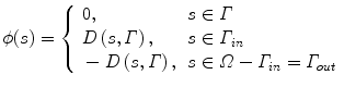
×  defined at a plane Ω. The most general form of the snake model consists of:
(1)
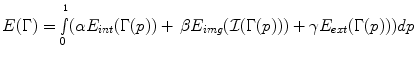
 is the input image, E int [=w1 |Γ′| + w 2 |Γ″ |] imposes smoothness constraints (smooth derivatives), E img [= − |∇
 |] makes the curve to be attracted from the image features (strong edges), E ext encodes either user interaction or prior knowledge and α, β, γ are coefficients that balance the importance of these terms.
The calculus of variations can be used to optimise such a cost function. To this end, a certain number of control points are selected along the curve, and the their positions are updated according to the partial differential equation that is recovered through the derivation of E(Γ) at a given control point of Γ. In the most general case a flow of the following nature is recovered:
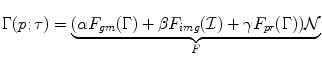
where  is the inward normal and F gm depends on the spatial derivatives of the curve, the curvature, etc. On the other hand, F img is the force that connects the propagation with the image domain and F pr (Γ) is a speed term that compares the evolving curve with a prior and enforces similarity with such a prior. The tangential component of this flow has been omitted since it affects the internal position of the control points and doesn’t change the form of the curve itself.
(2)
is the inward normal and F gm depends on the spatial derivatives of the curve, the curvature, etc. On the other hand, F img is the force that connects the propagation with the image domain and F pr (Γ) is a speed term that compares the evolving curve with a prior and enforces similarity with such a prior. The tangential component of this flow has been omitted since it affects the internal position of the control points and doesn’t change the form of the curve itself.Such an approach refers to numerous limitations. The number and the sampling rule used to determined the position of the control points can affect the final segmentation result. The estimation of the internal geometric properties of the curve is also problematic and depends on the sampling rule. Control points move according to different speed functions and therefore a frequent re-parameterisation of the contour is required. Last, but no least the evolving contour cannot change the topology and one cannot have objects that consist of multiple components that are not connected.
2.1 Level Set Method
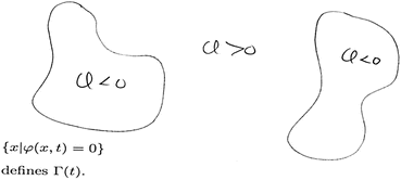
The level set method was first introduced in [10] and re-invented in [24] to track moving interfaces in the community of fluid dynamics and then emerged in computer vision [3, 21]. The central idea behind these methods is to represent the (closed) evolving curve Γ with an implicit function ϕ that has been constructed as follows:
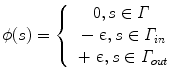 where epsilon is a positive constant, Γ in the area inside the curve and Γ out the area outside the curve as shown in [Fig. (1)]. Given the partial differential equation that dictates the deformation of Γ one now can derive the one for ϕ using the chain rule according to the following manner:
(3)
Fig. 1
Level set method and tracking moving interfaces; the construction of the (implicit) ϕ function [figure is courtesy of S. Osher]
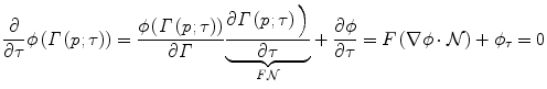
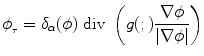
Let us consider the arc-length parameterisation of the curve Γ(c). The values of ϕ along the curve are 0 and therefore taking the derivative of ϕ along the curve Γ will lead to the following conditions:
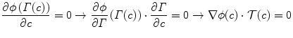
where  (c) is the tangential vector to the contour. Therefore one can conclude that ∇ϕ is orthogonal to the contour and can be used (upon normalisation) to replace the inward normal
 ![$$ \left[\mathcal{N}=-\frac{\nabla \phi}{\left|\nabla \phi \right|}\right] $$](/wp-content/uploads/2016/09/A151032_1_En_3_Chapter_IEq1.gif) leading to the following condition on the deformation of ϕ:
leading to the following condition on the deformation of ϕ:
Such a flow establishes a connection between the family of curves Γ that have been propagated according to the original flow and the ones recovered through the propagation of the implicit function ϕ. The resulting flow is parameter free, intrinsic, implicit and can change the topology of the evolving curve under certain smoothness assumptions on the speed function F. Last, but not least, the geometric properties of the curve like its normal and the curvature can also be determined from the level set function [24]. One can see a demonstration of such a flow in [Fig. (2)].
(4)
(c) is the tangential vector to the contour. Therefore one can conclude that ∇ϕ is orthogonal to the contour and can be used (upon normalisation) to replace the inward normal leading to the following condition on the deformation of ϕ:(5)
Fig. 2
Demonstration of curve propagation with the level set method; handling of topological changes is clearly illustrated through various initialization configurations (a,b,c)
In practice, given a flow and an initial curve the level set function is constructed and updated according to the corresponding motion equation in all pixels of the image domain. In order to recover the actual position of the curve, the marching cubes algorithm [20] can be used that is seeking for zero-crossings. One should pay attention on the numerical implementation of such a method, in particular on the estimation of the first and second order derivatives of ϕ, where the ENO schema [24] is the one to be considered. One can refer to [36] for a comprehensive survey of the numerical approximation techniques.
In order to decrease computational complexity that is inherited through the deformation of the level set function in the image domain, the narrow band algorithm [7] was proposed. The central idea is update the level set function only within the evolving vicinity of the actual position of the curve. The fast marching algorithm [35, 40] is an alternative technique that can be used to evolve curves in one direction with known speed function. One can refer to earlier contribution in this book [Chap. 7] for a comprehensive presentation of this algorithm and its applications. Last, but not least semi-implicit formulations of the flow that guides the evolution of ϕ were proposed [12, 42] namely the additive operator splitting. Such an approach refers to a stable and fast evolution using a notable time step under certain conditions.
2.2 Optimisation and Level Set Methods
The implementation of curve propagation flows was the first attempt to use the level set method in computer vision. Geometric flows or flows recovered through the optimisation of snake-driven objective functions were considered in their implicit nature. Despite the numerous advantages of the level set variant of these flows, their added value can be seen as a better numerical implementation tool since the definition of the cost function or the original geometric flow is the core part of the solution. If such a flow or function does not address the desired properties of the problem to be solved, its level set variant will fail. Therefore, a natural step forward for these methods was their consideration in the form of an optimisation space.
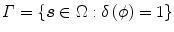
Such a framework was derived through the definition of simple indicator functions as proposed in [44] with the following behaviour
Once such indicator functions have been defined, an evolving interface Γ can be considered directly on the level set space as
while one can define a dual image partition using the  indicator functions as:
(6)
(7)
indicator functions as: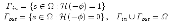
(8)
 ] , as well as well-defined derivatives [δ] in the entire domain a more appropriate selection was proposed in [44], namely the Dirac and the Heaviside distribution:
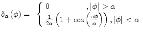
(9)
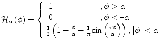
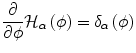
(10)
3 Data-driven Segmentation
The first attempt to address such task was made in [21] where a geometric flow was proposed to image segmentation. Such a flow was implemented in the level set space and aimed to evolve an initial curve towards strong edges constrained by the curvature effect. Within the last decade numerous advanced techniques have taken advantage of the level set method for object extraction.
3.1 Boundary-based Segmentation
The geodesic active contour model [4, 17] – a notable scientific contribution in the domain – consists of
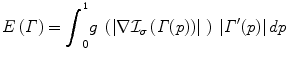
where  is the output of a convolution between the input image and a Gaussian kernel and
  is a decreasing function of monotonic nature. Such a cost function seeks a minimal length geodesic curve that is attracted to the desired image features, and is equivalent with the original snake model once the second order smoothness component was removed. In [4] a gradient descent method was used to evolve an initial curve towards the lowest potential of this cost function and then was implemented using the level set method.
(11)
is the output of a convolution between the input image and a Gaussian kernel and is a decreasing function of monotonic nature. Such a cost function seeks a minimal length geodesic curve that is attracted to the desired image features, and is equivalent with the original snake model once the second order smoothness component was removed. In [4] a gradient descent method was used to evolve an initial curve towards the lowest potential of this cost function and then was implemented using the level set method.A more elegant approach is to consider the level set variant objective function of the geodesic active contour;
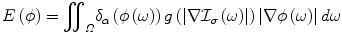
where Γ is now represented in an implicit fashion with the zero-level set of ϕ. One can take take the derivative of such a cost function according to ϕ:
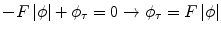
where ω and |∇  σ (ω)| were omitted from the notation. Such a flow aims to shrink an initial curve towards strong edges. While the strength of image gradient is a solid indicator of object boundaries, initial conditions on the position of the curve can be issue. Knowing the direction of the propagation is a first drawback (the curve has either to shrink or expand), while having the initial curve either interior to the objects or exterior is the second limitation. Numerous provisions were proposed to address these limitations, some of them aimed to modify the boundary attraction term [29], while most of them on introducing global regional terms [45].
(12)
(13)
σ (ω)| were omitted from the notation. Such a flow aims to shrink an initial curve towards strong edges. While the strength of image gradient is a solid indicator of object boundaries, initial conditions on the position of the curve can be issue. Knowing the direction of the propagation is a first drawback (the curve has either to shrink or expand), while having the initial curve either interior to the objects or exterior is the second limitation. Numerous provisions were proposed to address these limitations, some of them aimed to modify the boundary attraction term [29], while most of them on introducing global regional terms [45].3.2 Region-based Segmentation
In [26] the first attempt to integrate edge-driven and region-based partition components in a level set approach was reported, namely the geodesic active region model. Within such an approach, the assumption of knowing the expected intensity properties (supervised segmentation) of the image classes was considered. Without loss of generality, let us assume an image partition in two classes, and let r in ( ), r out (
 ) be regional descriptors that measure the fit between an observed intensity
  and the class interior [r in (
 )] and exterior to [r out (
 )] the curve. Under such an assumption one can derive a cost function that separates the image domain into two regions:
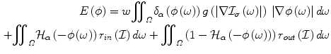
where w is a constant balancing the contributions of the two terms. One can see this framework as an integration of the geodesic active contour model [4] and the region-based growing segmentation approach proposed in [45]. The objective is to recover a minimal length geodesic curve positioned at the object boundaries that creates an image partition that is optimal according to some image descriptors. Taking the partial derivatives with respect to ϕ, one can recover the flow that is to be used towards such an optimal partition:
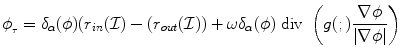
where the term δ α (−ϕ) was replaced with δ α (ϕ) since it has a symmetric behaviour. In [26] such descriptor function was considered to be the -log of the intensity conditional density [p in ( ), p in (
 )] for each class
), r out () be regional descriptors that measure the fit between an observed intensity and the class interior [r in ()] and exterior to [r out ()] the curve. Under such an assumption one can derive a cost function that separates the image domain into two regions:
according to a minimal length geodesic curve attracted by the regions boundaries,
according to an optimal fit between the observed image and the expected properties of each class,
(14)
(15)
), p in ()] for each class