Quantifying PET
Cyrill Burger
Alfred Buck
Although subjective reading of positron emission tomography (PET) images is still the basis of clinical diagnosis, strategies to extract quantitative information of disease processes will permit more objective diagnosis and comparisons among patient groups. Some quantification methods require the measurement of the true concentration of the tracer in tissue. Such data can be acquired only with a PET system that is correctly calibrated and routinely maintained.
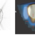
The aim of lesion quantification is to calculate an index related to the severity of the lesion. To this end, a volume of interest is generally defined around the lesion, and the average pixel value calculated (see Fig. 11.1). In doing this, a problem called the partial-volume effect occurs. Because of the limited spatial resolution of the PET system, the actual activity distribution becomes distorted. Depending on whether a lesion takes up more or less tracer than the surroundings, the true tracer concentration is underestimated or overestimated at the edges. A semiquantitative index often used for brain tumors is the lesion-to-reference ratio, which uses, for example, normal white matter as the reference tissue. The advantage of the method is the general availability of the internal standard and the removal of many distortion effects by the operation of division.
An index that has become popular during the last years for fluorodeoxyglucose (FDG) studies and is used for tumor grading is the standardized uptake value (SUV). In the initial definition, the tissue FDG concentration was normalized by the injected dose per gram body mass. Criticism led to the refinement of the SUV definition by replacing the total body mass by some measure of the lean body mass. The recommended way to measure lean body mass is using a fat and body weight scale rather than deriving it by an anthropometric formula. It is important to note that FDG uptake is not representative of the metabolic rate of glucose due to the potential change of the lumped constant in lesions. In some situations, patient images can be compared against the standard uptake pattern of normal controls to detect lesions and derive a quantitative measure of disease. A recent example is the fully automatic discrimination of patients with suspected Alzheimer dementia from normal controls on the basis of FDG data.
Introduction
In most situations, positron emission tomography (PET) imaging is done just like any other imaging modality. Images are acquired, reconstructed, and then reviewed with the aim of identifying pathologic lesions. Once a lesion is found, the decision about the lesion’s significance is based mainly on a visual comparison of its uptake with that of tissue considered to be normal, qualified by the physician’s experience. In this process, the numbers attributed to the lesion pixels by the reconstruction algorithm do not matter. Such relative assessments have been proven to be successful in clinical diagnostic routine, but they do not permit comparison between studies. This can be done with several more or less quantitative approaches. They allow comparison of the data for a patient group in order to arrive at a certain measure of the disease process (e.g., malignancy) or to assess numerically a therapy-induced effect in follow-up studies. Furthermore, they are mandatory for many types of research studies in which a baseline image is compared with an image in a specific condition, such as the brain perfusion before climbing Mount Everest and afterward (a study actually done in our PET center).
Calibration and Quality Control
As quantitative analyses require the reconstructed values in the image pixels, these have to be calibrated in absolute values to reflect the true tracer activity concentration in
kilobecquerels per cubic centimeter (kBq/cc) of the imaged tissue. To this end, a whole sequence of procedures must be performed (see Chapter 3). First, the procedures correct for the different types of signal distortions occurring during an acquisition, such as event losses due to detector dead time and photon attenuation, wrong “random” and scattered events, and differences in detector properties. With these corrections, true scanner “counts” represent the number of signals detected from each resolved tissue voxel. However, different scanners have different sensitivities for activity in the field of view, resulting in different count images for the same tracer distribution. Therefore, a calibration measurement must be performed with a homogeneous phantom (usually a cylinder containing a fluorine 18 [18F] solution of known activity concentration). The ratio of activity concentration to reconstructed counts represents the calibration factor that transforms the count image into a quantitative activity–concentration image in kilobecquerels per cubic centimeter. As the sensitivity varies among slices, one calibration factor per slice is applied. Because correct calibration is vital for quantitative analyses, quality control procedures must be performed on a regular basis, and the calibration repeated according to a schedule and after every significant system maintenance.
kilobecquerels per cubic centimeter (kBq/cc) of the imaged tissue. To this end, a whole sequence of procedures must be performed (see Chapter 3). First, the procedures correct for the different types of signal distortions occurring during an acquisition, such as event losses due to detector dead time and photon attenuation, wrong “random” and scattered events, and differences in detector properties. With these corrections, true scanner “counts” represent the number of signals detected from each resolved tissue voxel. However, different scanners have different sensitivities for activity in the field of view, resulting in different count images for the same tracer distribution. Therefore, a calibration measurement must be performed with a homogeneous phantom (usually a cylinder containing a fluorine 18 [18F] solution of known activity concentration). The ratio of activity concentration to reconstructed counts represents the calibration factor that transforms the count image into a quantitative activity–concentration image in kilobecquerels per cubic centimeter. As the sensitivity varies among slices, one calibration factor per slice is applied. Because correct calibration is vital for quantitative analyses, quality control procedures must be performed on a regular basis, and the calibration repeated according to a schedule and after every significant system maintenance.
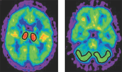 Figure 11.1 Volume-of-interest (VOI) definition in MCN-5652 data. Shown are two slices containing four VOIs in the putamen and the cerebellum. The pixels within the VOIs are assumed to represent homogeneous tissue. |
Distortion Effects
In most numeric analyses, the PET signal is averaged over a set of image pixels (a “volume of interest” [VOI], Fig. 11.1), based on the assumption that they represent homogeneous tissue. With such VOI methods, a problem arises related to the limited resolution of PET: the generation of so-called partial-volume effects (known also in CT and MR). An ideal imaging system would acquire perfect images of object shapes. Real systems, however, have a limited resolution and thus produce blurred images. The process of unsharp imaging can be modeled by a convolution of the true image with a function representing the impulse response, typically in the form of a Gaussian function. This function represents the characteristics of the imaging system, and its full width at half maximum (FWHM) is often used to define the resolution. PET systems typically have a resolution of approximately 5 to 10 mm in clinical imaging, so considerable blurring occurs.
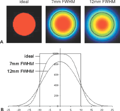 Figure 11.2 Partial-volume effect due to finite system resolution. A: A circular object of 20-mm diameter imaged with systems of ideal resolution (left), 7-mm full width at half maximum (FWHM; center), and 12-mm FWHM (right). B: Intensity profiles across the center of the images are overlaid in one diagram. |
Figure 11.2 illustrates the effect for a 20-mm-diameter synthetic hot lesion containing a count per pixel of 1,000 imaged with three systems. The perfect system yields the true image, and the second and third systems yield the true image convolved with a 7-mm and 12-mm Gaussian function. Applying a circular VOI of 20 mm to the images results in average pixel values of 1,000, 761, and 603, respectively. The reason for this progressive loss is obvious from the profiles in Figure 11.2B: a part of the activity is smeared to the neighborhood of the hot lesion. The loss is described by the “recovery coefficient,” which is defined as the fraction of the true counts that is measured in a VOI analysis. In the examples given, the recovery coefficients are 76.1% and 60.3%.
The recovery coefficient depends on several factors, such as the object size, the VOI size, the resolution of the scanner, and the lesion-to-background ratio. If a lesion takes up fewer trace than the surrounding tissue, the actual tracer concentration will be overestimated at the edges. An approach to reducing the partial-volume effect in lesions that are hotter than the surroundings is to use the maximum pixel value in the VOI instead of the pixel average (1). The advantage is that the impact of the partial-volume effect and of the VOI geometry, such as shape, size, and location, is greatly reduced.
Related posts:
 11C-Based PET- Radiopharmaceuticals of Clinical Value
 Brain Tumors: Astrocytoma, Oligodendroglioma, and Glioblastoma Images with PET and SPECT
 Sentinel Node Imaging in Head and Neck Tumors
 PET-CT and SPECT-CT of Bone Metastases
 SPECT and PET in Benign Thyroid and Parathyroid Disease
Stay updated, free articles. Join our Telegram channel

Full access? Get Clinical Tree


