Quantifying SPECT
David R. Gilland
Timothy G. Turkington
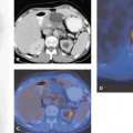
Single-photon emission computed tomography (SPECT) produces images that represent the distribution of radionuclides in the body. The accuracy with which the images represent these radionuclide concentrations depends on a variety of factors. In most clinical SPECT applications, the images are interpreted only qualitatively. Applications such as dosimetry measurements, tracking of tumor uptake over time, and kinetic analysis of radiotracer, however, require quantitative measurements of the radiotracer distribution in the body. To produce quantitative measurements with SPECT, it is necessary to understand and correct for the physical factors that affect the transport and detection of photons emitted by the radionuclides. These factors include attenuation (see Fig. 12.1), scatter, and spatial resolution effects (primarily from the collimator). Techniques have been developed to compensate for these effects, resulting in SPECT images that represent the radionuclide distribution in the body with quantitative accuracy. The final step in making quantitative measurements is accurate assignment of pixels to regions of interest, as in positron emission tomography (PET) imaging.
Introduction
In single-photon emission computed tomography (SPECT) imaging, the term “quantitation” has taken on many meanings. In all cases, the goal is to produce from the SPECT data not only a visual image of the radionuclide distribution but also a number that describes some underlying parameter represented by image. The particular aspect of the image that the number describes has been wide ranging and is the source of the many meanings of “quantitation.”
For our purposes, “SPECT quantitation” refers to using SPECT imaging methods to measure the detected count rate from a “feature” of interest within the image, such as a tumor or organ. This detected count rate typically is then used to compute a functional parameter of the image feature. “SPECT quantitation” also can refer to the measurement of the feature size (length, area, or volume).
The detected count rate of an image feature usually does not, by itself, provide meaningful physiologic information, but it does when compared with the count rate in another image or in a different region of the same image. For example, in tumor imaging, a change in detected count rate over time can indicate the response of the tissue to a drug or radiation therapy. In myocardial perfusion imaging, the ratio of the lung count rate to the myocardium count rate has been used as an indicator of cardiac function. In gated blood pool imaging, the ratio of the count in the ventricle at end diastole to that at end systole is used to compute ejection fraction and stroke volume. We can refer to these clinical applications as relative SPECT quantitation.
Relative quantitation can provide important physiologic information, but in some contexts it is important to know the absolute amount of radioactivity in the tissue. A prime application of this occurs in the area of radiation dosimetry. To calculate the radiation dose to organs of interest, the SPECT image must provide information on the total activity (e.g., μCi or MBq) in the image feature. Another application of absolute SPECT quantitation occurs in kinetic modeling. In this case, the goal is to compute functional parameters of an organ (e.g., blood flow) based on the SPECT-measured absolute activity concentration and activity measured from blood samples obtained over time. Here we focus on absolute SPECT quantitation.
Absolute SPECT quantitation is performed in two separate steps: (a) generation of a quantitatively accurate reconstructed SPECT image and (b) definition of the boundary of the feature of interest (i.e., segmentation of the image) and computation of its activity. The goal of the first step is to obtain a SPECT image in which the intensity of each voxel represents the true activity concentration within the body at that point. The goal of the second step is
compute the activity from within the feature of interest only, excluding activity from background regions. Both of these steps are critical for the accuracy of the overall SPECT quantitation.
compute the activity from within the feature of interest only, excluding activity from background regions. Both of these steps are critical for the accuracy of the overall SPECT quantitation.
Quantitative SPECT Reconstruction
SPECT quantitation requires a reconstructed image that accurately represents the rate of photon emission, or activity, per unit volume throughout the imaging field of view. Because it is impossible to detect all of the photons emitted at all points in the field of view, a calibration factor is required to relate the rate of photon detection to the rate of photon emission at all points of interest. In this section, we (a) summarize the important physical factors that affect SPECT quantitation and give examples of correction methods, (b) describe methods for calibrating the SPECT image for absolute activity quantitation, and (c) describe in greater depth current methods for compensating for an important factor in SPECT quantitation, attenuation.
Physical Factors Affecting SPECT Quantitation
A large number of physical factors can affect the SPECT quantitation of a particular image feature (1), but three factors stand out: attenuation, scatter, and detector response (or finite spatial resolution limited by the collimator). Other factors can play more prominent roles under special conditions (e.g., organ or patient motion and count losses due to detector dead time at high count rates), but these three are significant factors under most SPECT imaging conditions. Attenuation is the process whereby an emitted photon moving on a trajectory that would allow acceptance through the collimator undergoes a Compton interaction in body tissue and is deflected to a trajectory that is not accepted through the collimator. Scatter is a Compton interaction in body tissue with the opposite result: an emitted photon is deflected from a trajectory that would not allow acceptance to one that would. Thus attenuation removes counts from the detected image, whereas scatter adds counts, but adds them at the wrong position with respect to the point of emission. Detector response is the spatial blurring of image features, and its effect on SPECT quantitation is greatest for small features.
Attenuation
In most instances, attenuation has the greatest impact on SPECT quantitation and can result in order-of-magnitude errors if left uncorrected (4). This can be illustrated with the simple example of a point source at the center of a water-filled cylinder. For a 15-cm radius cylinder, the fraction of emissions (technetium 99m [99mTc]) not affected by attenuation is e(-μ × 15), where μ is the linear attenuation coefficient of water at 140 keV, or 0.151/cm. Thus attenuation results in almost a 90% decrease in reconstructed intensity at that point. For distributed sources, the effect is more complicated to analyze but can be illustrated with a slightly more complicated example: a uniform source distribution within the same cylinder. In this case, a profile through the resulting reconstructed image with and without attenuation correction is shown in Figure 12.1. As the figure shows, the reconstructed intensity without attenuation correction is erroneously small throughout the image but particularly so near the center of the cylinder. In more complicated (and more realistic) situations in which the body has nonuniform attenuating characteristics, more complicated artifacts result. The general trend still holds, however: deeper features are affected more by attenuation. Attenuation-correction methods are addressed later.
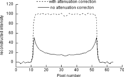 Figure 12.1 Effect of attenuation for a cylinder containing a uniform activity spread throughout. Note the marked central reduction in intensity (or activity) measured. |
Scatter
Scatter effects are more difficult to analyze than attenuation effects, but they are much smaller in magnitude. Typically, scatter results in an approximate 30% increase in detected counts compared with an idealized case in which scatter was excluded. This percentage will vary with the size of the attenuating medium. Many scatter-correction methods have been proposed for SPECT. The methods vary greatly in the extent of physical modeling that is used; however, a relatively simple method has been shown to reduce scatter effects effectively (2). The method uses data acquired within a second, lower-energy window. These “scatter” data, after appropriate scaling, are assumed to represent the scatter component of the primary energy window data and are subtracted from the primary energy window data. Because this method uses two energy windows, it is often referred to as the “dual-energy window method.”
Detector Response
Detector response, or finite spatial resolution, becomes an increasingly important factor in SPECT quantitation as the image feature size decreases. It is observed that for features smaller than approximately twice the spatial resolution of
the detector, the measured activity concentration decreases with the volume of the feature (3). The reason for this effect is that the detected counts in the SPECT image are spread across a larger region than that occupied by the emission source. Thus the measured concentration is necessarily reduced (see also Chapter 11). For larger sources, the spreading of counts away from a point in the SPECT image is balanced by the spreading into the point from surrounding areas of activity. Effective methods for detector-response correction involve linear deconvolution filtering with, for example, Wiener or Metz filters. An example of a Metz filter is shown in Figure 12.2. The filter exceeds unity gain at low spatial frequencies to deconvolve, or sharpen, the detector response blurring. The filter “rolls-off” to zero gain at high frequencies to control high-frequency image noise.
the detector, the measured activity concentration decreases with the volume of the feature (3). The reason for this effect is that the detected counts in the SPECT image are spread across a larger region than that occupied by the emission source. Thus the measured concentration is necessarily reduced (see also Chapter 11). For larger sources, the spreading of counts away from a point in the SPECT image is balanced by the spreading into the point from surrounding areas of activity. Effective methods for detector-response correction involve linear deconvolution filtering with, for example, Wiener or Metz filters. An example of a Metz filter is shown in Figure 12.2. The filter exceeds unity gain at low spatial frequencies to deconvolve, or sharpen, the detector response blurring. The filter “rolls-off” to zero gain at high frequencies to control high-frequency image noise.
Related posts:
 11C-Based PET- Radiopharmaceuticals of Clinical Value
 Brain Tumors: Astrocytoma, Oligodendroglioma, and Glioblastoma Images with PET and SPECT
 Sentinel Node Imaging in Head and Neck Tumors
 PET-CT and SPECT-CT of Bone Metastases
 SPECT and PET in Benign Thyroid and Parathyroid Disease
Stay updated, free articles. Join our Telegram channel

Full access? Get Clinical Tree


