Radiography involves the production of a two-dimensional image from a three-dimensional object, the patient (Fig. 7-1). The procedure projects the x-ray shadows of the patient’s anatomy onto the image receptor and is often called projection radiography. The source of radiation in the x-ray tube is a small spot, and x-rays that are produced in the x-ray tube diverge as they travel away from this spot. Because of beam divergence, the collimated x-ray beam becomes larger in area and less intense with increasing distance from the source. Consequently, x-ray radiography results in some magnification of the object being radiographed. Radiography is performed with the x-ray source on one side of the patient, and the image receptor is positioned on the other side of the patient. During the exposure, incident x-rays are differentially attenuated by anatomical structures in the patient. A small fraction of the x-ray beam passes unattenuated through the patient and is recorded on the image receptor, forming the latent radiographic image.
Although the principles in this chapter are described in terms of general radiography, they apply to other forms of medical imaging including mammography, fluoroscopy and interventional imaging, and the projection images acquired for planning computed tomographic examinations.
7.1 GEOMETRY OF PROJECTION RADIOGRAPHY
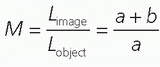
The geometry of projection transmission imaging is described in Figure 7-2. Magnification can be defined simply as
▪ FIGURE 7-1 The basic geometry of radiographic imaging is illustrated. The patient is positioned between the x-ray tube and the image receptor (A), and the radiograph is acquired. The ion chamber (shown between the grid and image receptor) determines the correct exposure level to the image receptor (automatic exposure control). In transmission imaging (B), the x-rays pass through each point in the patient, and the absorption of all the structures along each ray path combine to produce the primary beam intensity at that location on the image receptor. The signal level at each point in the image (C) reflects the degree of x-ray beam attenuation across the image. For example, the gray scale under the red dot on (C) corresponds to the total beam attenuation along the red line shown in (B).
▪ FIGURE 7-2 The geometry of beam divergence is shown. The object is positioned a distance a from the x-ray source, and the image receptor is positioned a distance (a + b) from the source. From the principle of similar triangles, the magnification, .
where Limage is the length of the object as seen on the image and Lobject is the actual length of the object. Due to similar triangles, the object magnification can be computed using the source to object distance (a) and the object to receptor distance (b)
The magnification will always be greater than 1.0 but approaches 1.0 when a relatively thin object (such as a hand in radiography) is positioned in contact with the detector, where b ≈ 0. The magnification factor changes slightly for each plane perpendicular to the x-ray beam axis, also known as the central ray, and thus anatomical structures at different depths in the patient are magnified differently. This characteristic means that, especially for thicker body parts, an AP (anterior-posterior) image of a patient will have a subtly different appearance to an experienced viewer than a PA (posterior-anterior) image of the same patient. Knowledge of the magnification in radiography is sometimes required clinically, for example, in angioplasty procedures where the diameter of the vessel must be measured to select the correct size of a stent or angiographic balloon catheter. In these situations, an object of known dimension (e.g., a catheter with notches at known spacing) is placed near the anatomy of interest, so that the magnification can be determined and a correction factor calculated.
Radiographic detectors should be exposed to x-ray intensities within a relatively small range. X-ray technique factors such as the applied tube voltage (kV), tube current (mA), and exposure time will be discussed later, but an important parameter that should be kept consistent is the distance between the x-ray source and the image receptor. For most radiographic examinations, the source-to-image distance (SID) is fixed at 100 cm (40 inches), and there are usually detents in the radiographic equipment that help the technologists to set this distance. Upright chest radiography is an exception, where the SID is typically set to 183 cm (72 inches). The larger SID used for chest radiography reduces the differential magnification in the lung parenchyma. Another consequence of projection of a three-dimensional object on a two-dimensional plane is that anatomic structures distant from the central ray experience differential magnification from those located near the central ray, even when they are at the same depth in the patient. This geometric distortion is more apparent for large body parts and short SID.
The focal spot in the x-ray tube is very small but is not truly a point source, resulting in magnification-dependent loss of resolution. The blurring from a finite x-ray source is dependent upon the geometry of the exam, as shown in Figure 7-3. The length of the edge gradient (Lg) is related to the length of the focal spot (Lf) by
where b/a represents the magnification of the focal spot. The edge gradient is measured using a highly magnified metal foil with a sharp edge. In most circumstances, higher object magnification increases the width of the edge gradient and reduces the spatial resolution of the image. Consequently, in most cases, the patient should be positioned with the anatomy of interest as close as possible to the image receptor to reduce magnification. For thin objects placed in contact with the image receptor, the magnification is approximately 1.0, and there will be negligible blurring caused by the finite dimensions of the focal spot. In some settings (e.g., mammography), a very small focal spot is used intentionally with magnification. In this case, the small focal spot produces much less magnification-dependent blur, and the projected image is larger as it strikes the image receptor. This intentional application of magnification radiography is used to overcome resolution limitations of the image receptor, and increases spatial resolution.
▪ FIGURE 7-3 The magnification of a sharp edge in the patient will cause blurring of that structure because the focal spot of the x-ray tube is not truly a point source. For a focal spot with width Lf, the intensity across this distributed source will affect how the edge is projected onto the image plane. The edge will no longer be perfectly sharp as shown in part B, but rather its shadow will reflect the source distribution as shown in part A. The intensity across the focal spot usually is approximately gaussian in shape, and thus the blurred profile of the edge will also appear gaussian. The length of the blur in the image is related to the width of the focal spot by .
As x-rays pass through the patient’s anatomy, they can interact by the fundamental physical processes of the photoelectric effect (PE) or Compton scatter, or they can continue on their way to the image receptor without interacting. X-rays that lose some of their energy through Compton scatter also usually change directions and can reach the image receptor divergent from the central ray. Typical image receptors have no means to discriminate between primary x-rays, which carry the important projection information, and secondary x-rays that tend to obscure the projection information. Therefore, methods are employed to restrict or minimize off-focus radiation from reaching the image receptor.
7.2 SCATTERED RADIATION IN PROJECTION RADIOGRAPHIC IMAGING
The basic principle of projection x-ray imaging is that x-rays travel in straight lines. However, when x-ray scattering events occur in the patient, the resulting scattered x-rays are not aligned with the trajectory of the original primary x-ray, and thus the straight-line assumption is violated (Fig. 7-4). Scattered radiation that does not strike the detector has no effect on the image; however, scattered radiation emanating from the patient is of concern for surrounding personnel due to the associated radiation dose. If scattered radiation is detected by the image receptor, it does have an effect on the image and can be a significant cause of image degradation. Scattered radiation generates image gray scale where it does not belong, and this can significantly reduce contrast. Contrast can be increased in digital images by window/leveling or other adjustment schemes, so for digital radiographic images, scatter acts chiefly as a source of noise, degrading the signal-to-noise ratio (SNR).
The amount of scatter detected in an image is characterized by the scatter-to-primary ratio (SPR) or the scatter fraction (F). The SPR is defined as the amount of energy deposited in a specific location in the detector by scattered photons, divided by the amount of energy deposited by primary (non-scattered) photons in that same location. Thus,
▪ FIGURE 7-4 X-rays scattered in the patient that reach the detector stimulate gray scale production, but since they are displaced on the image, they carry little or no information about the patient’s anatomy.
For an SPR of 1, half of the energy deposited on the detector at that location is from scatter—that is, 50% of the information in the image is largely useless. The scatter fraction is also used to characterize the amount of scatter, defined as
The relationship between the SPR and scatter fraction is given by
The vast majority of x-ray detectors integrate the x-ray energy and do not count photons, which is typical in nuclear medicine imaging. Thus, the terms S and P in this discussion refer to the energies absorbed in the detector from the scattered and primary photons, respectively.
If uncorrected, the amount of scatter on an image can be high (Fig. 7-5). The SPR increases typically as the volume of tissue that is irradiated by the x-ray beam increases. Figure 7-5 illustrates the SPR as a function of the side of a square field of view (FOV), for different patient thicknesses. The SPR increases as the field size increases and as the thickness of the patient increases. For a typical 30 × 30 abdominal radiograph in a 25-cm-thick patient, the SPR is about 4.5—so 82% (the scatter fraction) of the information in the image is essentially useless, if scatter rejection methods are not used.
7.2.1 The Antiscatter Grid
The antiscatter grid, or sometimes just called a scatter grid, is the most widely used technology for reducing scatter in radiography, fluoroscopy, and mammography. The grid is placed between the detector and the patient (Fig. 7-6). Ideally, it would allow all primary radiation incident upon it to pass, while absorbing all of the scattered radiation. The scatter grid has a simple geometric design, in which open interspace regions and alternating x-ray absorbing septa are aligned with the x-ray tube focal spot. This alignment allows x-ray photons emanating from the focal spot (primary radiation) to have a high probability of transmission through the grid, thereby reaching the detector, while more obliquely angled photons (scattered x-rays emanating from the interior of the patient) have a higher probability of striking the highly absorbing grid septa (Fig. 7-7). The alignment of the grid with the focal spot is crucial to its efficient operation, and errors in this alignment can reduce grid performance or cause artifacts in the image.
▪ FIGURE 7-5 The scatter-to-primary ratio (SPR) is shown as a function of the side dimension of a square field of view, for three different patient thicknesses. For example, the 15-cm point on the x-axis refers to a 15 × 15-cm field. The SPR increases with increasing field size and with increasing patient thickness. Thus, scatter is much more of a problem in the abdomen as compared to extremity radiography. Scatter can be reduced by aggressive use of collimation, which reduces the field of view of the x-ray beam.
▪ FIGURE 7-6 The antiscatter grid is located between the patient, who is the principal source of scatter, and the image receptor. Grids are geometric devices, and the interspace regions in the grid are aligned with the x-ray focal spot, which is the location from which all primary x-ray photons originate. Scattered photons are more obliquely oriented, and as a result have a higher probability of striking the attenuating septa in the grid. Hence, the grid allows most of the primary radiation to reach the image receptor, but prevents most of the scattered radiation from reaching it.
There are several parameters that characterize the antiscatter grid. For practical radiographic imaging in the clinical imaging environment, the following grid parameters are important:
7.2.2 Grid Ratio
The grid ratio is the most fundamental descriptor of the grid’s construction. The grid ratio (see Fig. 7-7) is the ratio of the height of the interspace material to its width—the septa dimensions do not affect the grid ratio metric. Grid ratios in general diagnostic radiology are most commonly 8, 10, or 12, with 6 or 14 used less often. Grid ratios are lower (˜5) in mammography. The grid septa in a grid are typically manufactured from lead (Z = 82, ρ = 11.3 g/cm3).
7.2.3 Interspace Material
Ideally, the interspace material would be air; however, the lead septa are very malleable and require support for structural integrity. Therefore, rigid material is placed in the interspace in the typical linear grid used in general radiography to keep the septa aligned. Low-cost grids in diagnostic radiology can have aluminum (Z = 13, ρ = 2.7 g/cm3) as the interspace material, but aluminum can absorb an appreciable number of the primary photons, especially at lower x-ray energies. Carbon fiber (Z = 6, ρ = 1.8 g/cm3) has high primary transmission due to the low atomic number of carbon and its lower density in fiber form, and thus is desirable as interspace material. Consequently, carbon fiber interspaced grids are more common in state-of-theart imaging systems.
▪ FIGURE 7-7 The basic dimensions of a 10:1 antiscatter grid are shown. The grid is comprised of alternating layers of interspace material and septa material. This illustration shows parallel grid septa; however, in a focused grid, the septa and interspace are pointed toward the expected location of the focal spot and thus would be slightly angled.
7.2.4 Grid Frequency
The grid frequency is the number of grid septa per centimeter. Looking at the grid depicted in Figure 7-7, the septa are 0.045 mm wide and the interspace is 0.120 mm wide, resulting in a line pattern with 0.165 mm spacing. The corresponding frequency is 1/0.165 mm = 6 lines/mm or 60 lines/cm. Grids with 70 or 80 lines/cm are also available, at greater cost. For imaging systems with discrete detector elements, a stationary high-frequency grid can be used. For example, a 2,048 × 1,680 chest radiographic system has approximately 200 µm detector elements, and thus a grid with 45-µm-wide grid septa (see Fig. 7-7) should ideally be invisible because the grid bars are substantially smaller than the spatial resolution of the detector. Even high-frequency grids can create patterns of non-uniformity in the image due to aliasing of the grid lines and the detector matrix. Unfortunate pairing of grids and detectors can cause pronounced artifacts, as can misalignment.
7.2.5 Grid Type
The grid pictured in Figure 7-7 is a linear grid, which is fabricated as a series of alternating septa and interspace layers. Grids with crossed septa are also available but seldom are used in general radiography applications. Crossed grids are widely used in mammography (Chapter 8).
7.2.6 Focal Length
The interspace regions in the antiscatter grid should be aligned with the x-ray source, and this requires that the grid be focused (see Fig. 7-6). The focal length of a grid is typically 100 cm for most radiographic suites and is 183 cm for most upright chest imaging units. If the x-ray tube is accidentally located at a different distance from the grid, then grid cutoff will occur. The focal distance of the grid is more forgiving for lower grid ratio grids, and therefore high grid ratio grids will have more grid cutoff if the source-to-detector distance is not exactly at the focal length. For systems where the SID can vary appreciably during the clinical examination (fluoroscopy), the use of lower grid ratio grids allows greater flexibility and will suffer less from off-focal grid cutoff, but will be slightly less effective in reducing the amount of scattered radiation that reaches the image receptor.
7.2.7 Moving Grids
Grids are located between the patient and the image receptor, and for high-resolution image receptors, the grid bars will be seen on the image if the grid is stationary. Stationary grids were common in upright screen-film chest radiography systems, and the success of this methodology suggests that radiologists are quite adroit at “looking through” the very regularly spaced grid lines on the image. A Bucky grid is a grid that moves with a reciprocating motion during the x-ray exposure, causing the grid bars to be blurred by this motion and not visible in the image. The motion is perpendicular to the long axis of the linear septa in the grid.
7.2.8 Bucky Factor
The Bucky factor, not to be confused with the moving Bucky grid, describes the relative increase in x-ray intensity or equivalently, mAs, needed when a grid is used, compared to when a grid is not used. The Bucky factor essentially describes the radiation dose penalty of using the grid—and typical values of the Bucky factor for abdominal radiography range from 3 to 8. The Bucky factor was critical for screen-film radiography, but is less germane to digital imaging systems. In screen-film radiography, the use of the grid slightly reduces the amount of detected primary radiation and substantially reduces the amount of scattered radiation detected, and both of these effects reduce the optical density (OD) of the resulting film. Thus, the x-ray technique has to be increased by the Bucky factor to replace this lost radiation, in order to produce films of the same OD. Digital systems, however, have much wider dynamic ranges than screen-film systems in general, and therefore the digital image can be amplified to compensate for the lower detected signal without increasing the x-ray technique. One could argue that the technique does not have to be increased to replace the scattered x-ray exposure to the detector, because it has no information content. However, the primary radiation that is blocked by the septa and interspace material would have contributed to the signal so it might be reasonable to increase the technique by the inverse of the primary transmission factor of the grid to maintain the SNR in the image. In practice, because screen-film image receptors enjoyed a century of clinical practice before being supplanted by digital imaging systems, the exposure factors used in digital systems largely follow the trends of what was used in the screen-film era. Nevertheless, these considerations suggest that digital radiography (DR) systems may be used to provide lower dose examinations than those in the screen-film radiography.
It is important to note that for thin anatomical structures, there is very little scattered radiation, and an antiscatter grid is unnecessary. For example, for hand or forearm radiography, scatter levels are low and the technologist will usually place the limb to be imaged directly on the detector, without a grid, if it is removable. Likewise, for pediatric patients often the body part thickness is small and scatter removal is unnecessary.
There are other parameters that characterize the performance of the antiscatter grid, which are used primarily in the scientific evaluation of grid performance. These parameters are less important to x-ray technologists and radiologists, but are of interest to those engaged in designing grids or optimizing their performance. These metrics are discussed below.
7.2.9 Primary Transmission Factor
Tp is the fraction of primary photons that are transmitted through the grid, and ideally it would be 1.0. In Figure 7-7, the grid bars cover 27% of the field (0.045/[0.045 + 0.120]) and primary x-rays striking the top of the septa (parallel to their long axis) will be mostly attenuated. For that grid, then, the primary transmission would at most be 73%, and this does not consider the attenuation of the interspace material. Values of Tp typically run from 0.50 to 0.75 with modern grids, and this value is kV-dependent due to the penetration of the interspace material. As mentioned above, this metric may be more germane to clinical radiography using digital image receptors than the Bucky factor.
7.2.10 Scatter Transmission Factor
Ts is the fraction of scattered radiation that penetrates the grid. Ideally, it would be 0. The value of Ts can range substantially depending on the amount of scatter in the field, the x-ray energy, and the grid design. Typical values of Ts range approximately from 0.05 to 0.20 in general diagnostic radiography.
7.2.11 Selectivity
Selectivity (Σ) is simply defined as the ratio between the transmission of primary and scattered radiation, hence,
7.2.12 Contrast Degradation Factor
The contrast degradation factor (CDF) refers to the reduction in contrast due to scattered radiation. It can be shown that contrast is reduced by
However, because digital images can be adjusted to enhance contrast, CDF is less critical in digital radiography than in film-screen radiography. However, this metric indicates the degree to which contrast must be adjusted to compensate for scatter.
7.2.13 Other Methods for Scatter Reduction
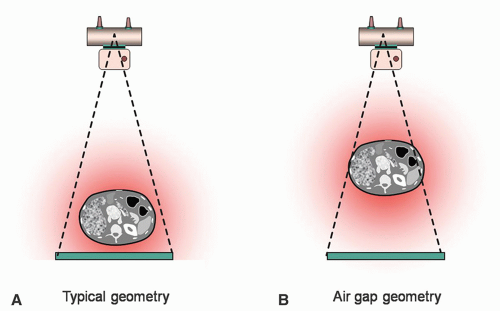
While the antiscatter grid is by far the most ubiquitous tool used for scatter reduction, air gaps and slot-scan techniques have been studied for years (Fig. 7-8). The principle of the air gap is that by moving the patient away from the image receptor, less of the scatter emitted from the patient will impinge on the image receptor. The concept is similar to the inverse square law, where radiation intensity decreases as the square of the distance from the source. However, scatter from the patient does not originate from a point, but instead from a large volume, and thus is an extended source of radiation. The scattered x-ray intensity decreases as the air gap distance increases proportional to 1/r, rather than 1/r2. Increasing the air gap distance also increases the magnification of the patient’s anatomy (see Fig. 7-2). Practical factors limit the utility of the air gap method for scatter reduction—as magnification of the patient anatomy increases, the coverage of a given detector dimension is reduced, there is a loss in spatial resolution due to the increased blurring of the finite focal spot with magnification (see Fig. 7-3), and the exposure technique may need to be increased if the overall SID is lengthened in order to maintain the same exposure level at the image receptor.
▪ FIGURE 7-8 The air gap technique has been used to reduce scattered radiation, and this figure shows the air gap geometry. The scattered radiation that might strike the image receptor in the typical geometry (A) has a better probability of not striking the image receptor as the distance between the patient and the image receptor is increased. B. While often discussed, the air gap technique suffers from limited field coverage and magnification issues, and is used only rarely in diagnostic radiography.
The slot-scan system for scatter reduction (Fig. 7-9) is one of the most effective ways of reducing the detection of scattered x-rays, and images produced from scanslot systems are often noticeably better in appearance due to their excellent contrast and SNR. Slot-scan radiography can be regarded as the gold standard in scatter reduction methods. The method works because a very small field is being imaged at any point in time (see Fig. 7-5), most scatter is prevented from reaching the image receptor, and the image is produced by scanning the small slot across the entire FOV. In addition to excellent scatter rejection, slot-scan radiography also does not require a grid and therefore has the potential to be more dose efficient. The dose efficiency of slot-scan systems is related to the geometric precision achieved between the alignment of the prepatient slit and the postpatient slot. If the postpatient slot is collimated too tightly relative to the prepatient slit, primary radiation that has passed through the patient will be attenuated, reducing dose efficiency. If the postpatient slot is too wide relative to the prepatient slit, then more scatter will be detected.
▪ FIGURE 7-9 The scanning slit (or “slot-scan”) method for scatter reduction is illustrated. The prepatient slit is aligned with the postpatient slot, and these two apertures scan across the field of view together. The challenge is to keep the slot aligned with the slit, and this can be done electronically or mechanically. This geometry was deployed for an early digital mammography system, but is also commercially available for radiography applications. Excellent scatter reduction can be achieved using this method.
Despite the excellent scatter reduction from these systems, the technology has inherent limitations compared to conventional large FOV radiography. The scanning approach requires significantly longer acquisition times, and the potential for patient motion during the acquisition increases. The narrow aperture for scanning requires a high x-ray tube current and the longer scan time causes significant heat loading of the x-ray tube anode. Alignment of mechanical systems is always a source of concern, and complex mechanical systems invariably require more attention from service personnel. These practical limitations have likely constrained the clinical success of slot-scan systems.
As mentioned above, the primary effect of scatter is to degrade contrast in the image. With digital image receptors, contrast can be modified by digital image processing so long as enough primary x-rays contribute to the image in order to maintain the SNR. Several commercial products have been introduced for substituting image processing for an actual physical antiscatter grid, mainly for bedside radiography. In bedside radiography, the short SID and non-compliant patient amplify the challenges of using an antiscatter grid. Misregistration of the grid with respect to the central ray of the x-ray beam, difficulty maintaining perpendicular alignment, and variability in SID can generate undesired non-uniformity or “grid washout” in the image. Clinically, this can cause one lung to appear dark and the other light, mimicking a pathological condition.
Restoring the contrast lost from scatter is not a simple process. The first step involves estimating the amount of scatter in the image. As noted previously, the amount of scatter produced depends on the volume of tissue in the x-ray beam. The software estimates the amount of scatter based on the output of the x-ray generator and the signal reaching the image receptor. From this information, the thickness of the patient is estimated. After the amount of scatter is estimated, the reduction of scatter expected from an actual physical antiscatter grid is estimated. Next, the proportion of scatter that was calculated to be removed by a physical grid is subtracted from the original image. Subsequent image processing may be applied to reduce noise or further modify contrast.
Although grid simulation appears to have promise for producing exceptional quality images without the dose penalty involved with physical grids, the technology has encountered some skepticism. Scatter is non-uniform across the FOV and depends on collimation and the anatomy included in the FOV, which is variable in bedside radiography. It is unclear how the software compensates for these variables in the scatter estimation step. The second step attempts to estimate the performance of a specific physical grid of the manufacturer’s choosing, which may not be similar to the one preferred by the clinical end user. The fundamental uncertainty when subtraction is applied to an image is how the algorithm determines what is noise and what is signal for the subtraction step. The error in this method is likely small for high-contrast features such as bone, but possibly greater for low-contrast soft tissue features. Unfortunately, some manufacturers employ a low kV and radiation dose to the detector that is similar to acquisition with a physical grid, compromising the advantage in patient radiation dose.
7.3 TECHNIQUE FACTORS IN RADIOGRAPHY
The principal x-ray technique factors used for radiography include the tube voltage (the kV), the tube current (mA), the exposure time, and the x-ray source-to-image distance, SID. The SID is standardized to 100 cm typically (Fig. 7-10) and 183 cm for upright chest radiography. In general, lower kV settings will increase the dose to the patient compared to higher kV settings for the same imaging procedure and same body part, but the trade-off is that subject contrast is reduced with higher kV. The kV is usually adjusted according to the examination type—lower kVs are used for bone imaging and when iodine or barium contrast agents are used; however, the kV is also adjusted to accommodate the thickness of the body part. For example, in bone imaging applications, 55 kV can be used for wrist imaging since the forearm is relatively thin, whereas 75 to 90 kV might be used for lumbar spine radiography, depending on the size of the patient’s abdomen. The use of the 55-kV beam in abdominal imaging would result in a prohibitively high radiation dose. Lower kVs emphasize contrast due to the photoelectric effect in the patient, which is important for higher atomic number (Z) materials such as bone (Zcalcium = 20) and contrast agents containing iodine (Z = 53) or barium (Z = 56). Conversely, for chest radiography, the soft tissues of the cardiac silhouette and pulmonary anatomy are of interest, and the ribs obscure them. In this case, high kV is used (typically 120 kV) in order to decrease the conspicuity of the ribs by reducing photoelectric interactions. While the anatomy of interest in the chest examination is soft tissue, the rib examination for the same FOV, uses lower kV to emphasize contrast of bony structures. Sometimes higher kV technique is selected irrespective of the loss of subject contrast, in order to increase the output of the x-ray tube and achieve a reasonable exposure at the image receptor in a reasonable exposure time to avoid patient motion during the exposure. In the example above, the 55 kV beam would require at least four times as long an exposure as the 75 kV beam at the same mA setting, without considering any differences in attenuation.
With the SID and kV adjusted as described above, the overall x-ray fluence is then adjusted by using the mA and the time (measured in seconds). The product of the mA and time (s) is called the mAs, and at the same kV and distance, the x-ray fluence is linearly proportional to the mAs—double the mAs, and the x-ray fluence doubles. Modern x-ray generators and tubes designed for radiography can operate at relatively high mA (such as 500 to 800 mA), and higher mA settings allow the exposure time to be shorter, which “freezes” patient motion. Some examinations, so-called breathing techniques, employ deliberately long exposure times to allow patient motion to blur anatomic features and emphasize features that would otherwise be obscured by overlying anatomy.
▪ FIGURE 7-10 The standard configuration for radiography is illustrated. Most table-based radiographic systems use a SID of 100 cm. The x-ray collimator has a light bulb and mirror assembly in it, and, when activated, casts a light beam onto the patient allowing the technologist to position the x-ray beam with respect to the patient’s anatomy. The light beam is congruent with the x-ray beam. X-rays that pass through the patient must also pass through the antiscatter grid and the ion chamber (part of the AEC system) in order to reach the image receptor.
Manual selection of x-ray technique, also called “fixed technique,” was used in radiography until the 1970s, whereby the technologist selected the kV and mAs based on experience and in-house “technique charts” (Table 7-1). The technique chart was considered by some to be the radiologist’s prescription for radiation exposure for the specified view. The technique chart was used in conjunction with the “protocol book,” a document that specifies the number and type of radiographic views that constitute an examination, and details of the FOV and anatomic markers of each view. Most examinations consist of one view where the x-ray beam is perpendicular to the anatomy and another orthogonal view. This is intended to allow the radiologist to visualize the anatomy in three dimensions. Examinations may include views from other angles such as oblique or decubitus views in order to present the anatomy of interest. Many institutions required technologists to use large calipers to measure the thickness of the body part to be imaged, to improve the consistency of the radiographic film OD.
Today, radiography usually relies on automatic exposure control (AEC), informally called phototiming because of an early device used for the same purpose. The mA is set to a high value such as 500 mA, and the exposure time (and hence the overall mAs) is determined by the AEC system. In general radiography, an air-ionization chamber is located behind the patient and grid, but in front of the x-ray detector (Fig. 7-10). During exposure, the AEC integrates the exposure signal from the ion chamber in real time until a preset exposure level is reached, and then the AEC immediately terminates the exposure. The preset exposure levels are calibrated by the service personnel, and the sensitivity of the radiographic detector is taken into account in the calibration procedure. For screen-film radiography, the AEC was set to deliver proper film darkening. For a digital radiographic system, the AEC is adjusted so that the exposure levels are both in the range of the detector system and produce images with good statistical integrity based on a predetermined SNR. This means that a trade-off between radiation dose to the patient and noise in the digital image should be reached. For some digital imaging systems, the signal from the detector itself can serve as the AEC sensor.
The reliance of technologists on AEC for exposure factor control gives rise to a number of problems, even for modern digital radiographic systems. First, the technique chart still exists; it is embedded in the modern x-ray operator console. It incorporates many assumptions about the size of the patient, usually segregated into six classes, namely large, medium, and small adult and pediatric patients. The technologist must make a determination of the size category of the patient, the default typically being medium adult. Incorrect assessment of patient size has consequences for the technique factors selected and often the postacquisition digital image processing. For example, if the mA setting is appropriate for a large patient, but the patient is actually small, the exposure time may be shorter than the response time of the AEC system (less than 5 ms), resulting in unintended overexposure. Second, most systems allow the technologist to perform the exposure out of the configuration called for by the technique guide, for example, excluding the antiscatter grid or acquiring at a different SID. This has consequences for image quality that may not be immediately obvious. Third, AEC assumes proper positioning of the patient with respect to the AEC sensor. If the dense anatomy such as bone is positioned in front of the active AEC sensor, the exposure time may be much longer than intended. If the AEC sensor is uncovered, that is, outside the shadow of the patient, the exposure time may be much shorter than intended resulting in a noisy, non-diagnostic image. There are usually multiple AEC sensors that can be selected independently or in groups. If the technologist activates the wrong sensors for a particular view, inappropriate exposure may be delivered. Finally, the computerized operator console in one room may not contain the same technique settings as an identical room next door. This causes unintended variability in the appearance of images.


 .
.


 .
.