apply a transformation defined by parameters  . In 2D, similarity transformations have 4 parameters, affine transformations are defined by 6 parameters. The configurations of points defined by
  and
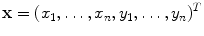
and  are considered to have the same shape. Shape differences are those changes that cannot be explained by application of such a global transformation. If we use n 2D points,
 , to describe the shape, then we can represent the shape as the 2n element vector,
  , where
(1)
For instance, Fig. 1 gives an example of a set of 46 points used to define the shape of the outline of a vertebra in a DXA image
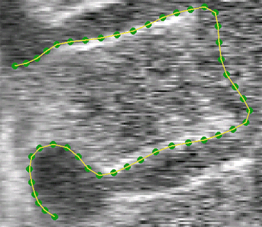
Fig. 1
Set of points used to define the shape of a vertebra in a DXA image (image enhanced to aid visibility of structures)
Given s training examples, we generate s such vectors  (
( ). Before we can perform statistical analysis on these vectors it is important that the shapes represented are in the same co-ordinate frame. This can be achieved by using Procrustes Analysis [15]. This transforms each shape in a set,
  , so that the sum of squared distances of the shape to the mean (
 ) is minimised.
(). Before we can perform statistical analysis on these vectors it is important that the shapes represented are in the same co-ordinate frame. This can be achieved by using Procrustes Analysis [15]. This transforms each shape in a set, , so that the sum of squared distances of the shape to the mean () is minimised.Let the vector  contain the n coordinates of the i th shape. These vectors form a distribution in 2n dimensional space.
contain the n coordinates of the i th shape. These vectors form a distribution in 2n dimensional space.If we can model this distribution, we can generate new examples, similar to those in the original training set, and we can examine new shapes to decide whether they are plausible examples.
To simplify the problem, we first wish to reduce the dimensionality of the data from nd to something more manageable. An effective approach is to apply Principal Component Analysis (PCA) to the data [10]. The data form a cloud of points in the 2n-D space. PCA computes the main axes of this cloud, allowing one to approximate any of the original points using a model with fewer than 2n parameters. The result is a linear model of the form

where  is the mean of the data,
  contains the t eigenvectors of the covariance matrix of the training set, corresponding to the largest eigenvalues,
  is a t dimensional parameter vector.
(2)
is the mean of the data, contains the t eigenvectors of the covariance matrix of the training set, corresponding to the largest eigenvalues, is a t dimensional parameter vector.Equation (2) generates a shape in the model frame, where the effects of the global transformation have been removed by the Procrustes Analysis. A shape in the image frame,  , can be generated by applying a suitable transformation to the points,
  :
:  . Typically
  will be a similarity transformation described by a scaling, s, an in-plane rotation,
  , and a translation
  .
.
, can be generated by applying a suitable transformation to the points, : . Typically will be a similarity transformation described by a scaling, s, an in-plane rotation, , and a translation .The best choice of parameters for a given shape  is given by
The vector  defines a set of parameters of a deformable model. By varying the elements of
  we can vary the shape,
  , using Eq. (2). The variance of the i th parameter, b i , across the training set is given by
  . By applying suitable limits to the model parameters we ensure that the shape generated is similar to those in the original training set.
is given by(3)
defines a set of parameters of a deformable model. By varying the elements of we can vary the shape, , using Eq. (2). The variance of the i th parameter, b i , across the training set is given by . By applying suitable limits to the model parameters we ensure that the shape generated is similar to those in the original training set.If the original data,  , is distributed as a multivariate Gaussian, then the parameters
  are distributed as an axis-aligned Gaussian,
  where
where  . In practise it has been found that the assumption of normality works well for many anatomical structures.
, is distributed as a multivariate Gaussian, then the parameters are distributed as an axis-aligned Gaussian, where . In practise it has been found that the assumption of normality works well for many anatomical structures.2.1 Examples of shape models
Figure 2 shows the effect of changing the first two shape parameters on a model of the outline of a vertebra, trained from 350 examples such as that shown in Fig. 1.
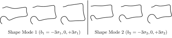
Fig. 2
First two modes of a shape model of a vertebra (Parameters varied by ± 3 s.d. from the mean)
Figure 3 shows the effect of varying the parameter controlling the first mode of shape variation of a 3D model of a set of deep brain structures, constructed from shapes extracted from MR images of 69 different subjects1. Note that since the method only represents points, it easily model multiple structures.
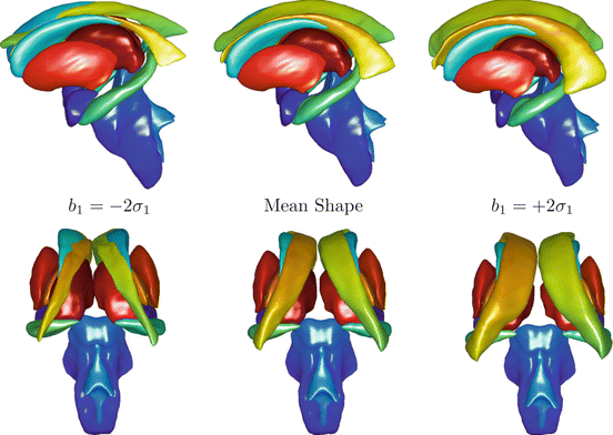
Fig. 3
Two views of the first mode of a shape model of structures in the brain
3 Active Shape Models
Given a new image containing the structure of interest, we wish to find the pose parameters,  , and the shape parameters,
  , which best approximate the shape of the object. To do this we require a model of how well a given shape would match to the image.
, and the shape parameters, , which best approximate the shape of the object. To do this we require a model of how well a given shape would match to the image.Suppose we have a set of local models, each of which can estimate how well the image information around a point matches that expected from the training set, returning a value  . We then seek the shape and pose parameters which generate points
  so as to maximise
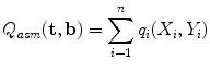
where 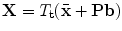 .
.
. We then seek the shape and pose parameters which generate points so as to maximise(4)
.The basic Active Shape Model algorithm is a simple iterative approach to locating this optima. Each iteration involves two steps
1.
Search around each point  for a better position,
for a better position, 2.
Update the pose and shape parameters to best fit the model to the new positions 
By decoupling the search and update steps the method can be fast. Since each point is searched for independently, it is simple to implement and can make use of parallel processing where available.
Because of the local nature of the search, there is a danger of falling into local minima. To reduce the chance of this it is common to use a multi-resolution framework, in which we first search at coarse resolutions, with low resolution models, then refine at finer resolutions as the search progresses. This has been shown to significantly improve the speed, robustness and final accuracy of the method.
The approach has been found to be very effective, and numerous variants explored. In the following we will summarise some of the more significant approaches to each step.
3.1 Searching for Model Points
The simplest approach is to have q i (X, Y ) return the edge strength at a point. However we will usually have a direction and scale associated with each point, allowing the local models to be more specific. For instance, since most points are defined along boundaries (or surfaces in 3D), the normal to the boundary/surface defines a direction, and a scale can be estimated from the global pose transformation.
Since we have a training set, a natural approach is to learn statistical models of the local structure from that around each point in the known examples [10]. For each model point in each image, we can sample at a set of nearby positions. For instance, at points along smooth curves we can sample profiles (Fig. 4a), whereas at corner points we can sample on a grid around the point (Fig. 4b).
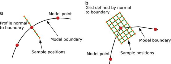
Fig. 4
ASM search requires models of the image around each point
The samples around model point i in training image j can be concatenated into a vector,  . Typically each such vector is normalised to introduce invariance to overall intensity effects (for instance, by subtracting the mean intensity and scaling so the vector is of unit length). We then can estimate the probability density distribution
  , which may be a Gaussian, or something more sophisticated if sufficient samples are available.
. Typically each such vector is normalised to introduce invariance to overall intensity effects (for instance, by subtracting the mean intensity and scaling so the vector is of unit length). We then can estimate the probability density distribution , which may be a Gaussian, or something more sophisticated if sufficient samples are available.Given such a PDF for each point, we can evaluate a new proposed position by sampling the image around the point into a new vector  , and setting
 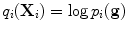 .
.
, and setting .To search for a better position, we evaluate the PDF at a number of displaced positions, and choose the best. For profile models, we typically search at positions along a profile normal to the current boundary. For grid based models, we would test points on a grid. There are natural extensions to 3D volume images.
Rather than simply sample image intensities, it is possible to sample other features. For instance van Ginneken et al. [36] sampled Gabor features at multiple scales.
This approach has been shown to be effective in many applications [10]. However, van Ginneken et al. [36] pointed out that improved estimates of the model point positions can be obtained by explicitly training classifiers for each point, to discriminate the correct position from incorrect nearby positions. The approach is to treat samples at the model points in the training set as positive examples, then create a set of negative examples by sampling nearby. These examples are used to train a classifier. During search samples around a set of candidate positions are evaluated, and the one most strongly classified as positive is used. It is assumed that the classifier gives a continuous response which is larger for positive examples, and can thus be used to rank the candidates.
In the case of [36] a nearest neighbour classifier was used, but encouraging results have been obtained with a range of methods. For instance, Li and Ito [37] used Adaboost to train a classifier for facial feature point detection.
A related approach is to attempt to learn an objective function which has its minimum at the correct position, and has a smooth form to allow efficient optimisation [28].
3.2 Updating the Model Parameters
After locating the best local match for each model point,  , we update the model pose and shape parameters so as to best match these new points. This can be considered as a regularisation step, forcing points to form a ‘reasonable’ shape – one defined by the original model.
, we update the model pose and shape parameters so as to best match these new points. This can be considered as a regularisation step, forcing points to form a ‘reasonable’ shape – one defined by the original model.The simplest approach is to find  and
and  so as to minimise
and so as to minimise(5)
For anything other than when T() is a translation, this is a non-linear sum of squares problem, so can be efficiently solved with Levenberg-Marquardt [29], or an iterative algorithm in which we alternate between solving for  with fixed
  , and solving for
  with fixed
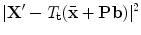
  , each of which has a closed form. To prevent the generation of extreme shapes, limits can be placed on the parameters. If we assume a normal distribution for the original shapes, then the parameters b i are linearly independent with a variance
  . A natural constraint is then to force
Since M will be distributed as  with t degrees of freedom, this distribution can be used to select a suitable value of M thresh (for instance, one that includes 98% of the normal samples).
with fixed , and solving for with fixed , each of which has a closed form. To prevent the generation of extreme shapes, limits can be placed on the parameters. If we assume a normal distribution for the original shapes, then the parameters b i are linearly independent with a variance . A natural constraint is then to force(6)
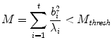
with t degrees of freedom, this distribution can be used to select a suitable value of M thresh (for instance, one that includes 98% of the normal samples).This approach effectively treats every choice of shape parameters within the threshold as equally likely. An alternative is to include a prior, rather than a hard threshold, for instance
where σ r 2 is the variance of the residuals (those not explained by the model) in the model frame and we assume all pose parameters are equally likely. We can thus find the most likely values for  by optimising (7). Again, this is a non-linear sum of squares problem, for which fast iterative algorithms exist (for instance, see [38]).
(7)
by optimising (7). Again, this is a non-linear sum of squares problem, for which fast iterative algorithms exist (for instance, see [38]).Information about the uncertainty of the estimates of the best matching point positions can also be included into the optimisation [17].
Since the models for each point may return false matches (for instance by latching on to the wrong nearby structure), it can be effective to use a more robust method in which outliers are detected and discarded [27].
4 Active Appearance Models
The Active Shape Model treats the search for each model point as independent. However, there will usually be correlations between the local appearance around nearby points. This can be modelled, but leads to a more difficult optimisation problem. The Active Appearance Model algorithm is a local optimisation technique which can match models of appearance to new images efficiently.
Related posts:

Stay updated, free articles. Join our Telegram channel

Full access? Get Clinical Tree


