Single Photon Emission Computed Tomography

Fig. 12.1

Four slices of the heart in the short axis

In nuclear medicine, two types of ECT have been in practice based on the type of radionuclides used: single photon emission computed tomography (SPECT) , which uses γ-emitting radionuclides such as ^99mTc, ¹²³I , ⁶⁷Ga , and ¹¹¹In, and positron emission tomography (PET) , which uses β⁺-emitting radionuclides such as ¹¹C , ¹³N , ¹⁵O , ¹⁸F , ⁶⁸Ga , and ⁸²Rb . SPECT is described in detail in this chapter and PET in Chap. 13.

Single Photon Emission Computed Tomography

The most common SPECT system consists of a typical gamma camera with one to three NaI(Tl) detector heads mounted on a gantry, an online computer for acquisition and processing of data, and a display system (Fig. 12.2). The detector head rotates around the long axis of the patient at small angle increments (3 to 10°) for collection of data over 180 or 360°. The data are collected in the form of pulses at each angular position and normally stored in a 64 × 64 or 128 × 128 matrix in the computer for later reconstruction of the images of the planes of interest. Note that the pulses are formed by the PM tubes from the light photons produced by the interaction of γ-ray photons from the object, which are then amplified, verified by X, Y position and PH analyses, and finally stored. Transverse (short axis), sagittal (vertical long axis), and coronal (horizontal long axis) images can be generated from the collected data. Multihead gamma cameras collect data in several projections simultaneously and thus reduce the time of imaging. For example, a three-head camera collects a set of data in about one third of the time required by a single-head camera for 360° data acquisition.

Fig. 12.2

A dual-head SPECT camera, e-CAM model (Courtesy of Siemens Medical Solutions, Hoffman Estates, IL).

Data Acquisition

The details of data collection and storage such as digitization of pulses, use of frame mode or list mode, choice of matrix size, etc., have been given in Chap. 11.

Data are acquired by rotating the detector head around the long axis of the patient over 180 or 360°. Although 180° data collection is commonly used (particularly in cardiac studies), 360° data acquisition is preferred by some investigators, because it minimizes the effects of attenuation and variation of resolution with depth. In 180° acquisition using a dual-head camera with heads mounted in opposition (i.e., 180°), only one detector head is needed for data collection and the data acquired by the other head essentially can be discarded. In some situations, the arithmetic mean (A₁ + A₂)/2 or the geometric mean (A₁ ´ A₂)^1/2 of the counts, A₁ and A₂, of the two heads are calculated to correct for attenuation of photons in tissue. However, in 180° collection, a dual-head camera with heads mounted at 90° angles to each other has the advantage of shortening the imaging time required to sample 180° by half (Table 12.1). Dual-head cameras with heads mounted at 90 or 180° angles to each other and triple-head cameras with heads oriented at 120° to each other are commonly used for 360° data acquisition and offer shorter imaging time than a one-head camera for this type of angular sampling.

Table 12.1

Relationship of sensitivity and time of imaging for 180 and 360° acquisitions for different camera head configurations

	180° Acquisition		360° Acquisition
Camera Type	Acquisition time (min)	Relative sensitivity	Acquisition time (min)	Relative sensitivity
Single-head	15	1	15	1
Dual-head (heads at 180°)	15	1	7.5	2
Dual-head (heads at 90°)	7.5	2	7.5	2
Triple-head (heads at 120°)	10	1.5	5	3

The sensitivity of a multihead system increases with the number of heads depending on the orientation of the heads and whether 180 or 360° acquisition is made. Table 12.1 illustrates the relationship among sensitivity, time of imaging, and acquisition arc (180 or 360°) for different camera head configurations.

Older cameras were initially designed to rotate in circular orbits around the body. Such cameras are satisfactory for SPECT imaging of symmetric organs such as the brain, but because the body contour is not uniform, such a circular orbit places the camera heads at different distances from various parts of the body in the anterior, lateral, and posterior positions. This causes loss of data and hence loss of spatial resolution in projections. To circumvent this problem, many modern cameras are designed to include a feature called noncircular orbit (NCO) (i.e., to follow the body contour) that moves the camera heads such that the detector remains at the same distance close to the body contour at all angles.

Data collection can be made in either continuous motion or “step-and-shoot” mode. In continuous acquisition, the detector rotates continuously at a constant speed around the patient, and the acquired data are later binned into the number of segments equal to the number of projections desired. In the step-and-shoot mode, the detector moves around the patient at selected incremental angles (e.g., 3°) and collects the data for the projection at each angle.

Image Reconstruction

Data collected in two-dimensional projections give planar images of the object at each projection angle. To obtain information along the depth of the object, tomographic images are reconstructed using these projections. Two common methods of image reconstruction using the acquired data are the backprojection method and the iterative method. Both methods are described below.

Simple Backprojection

The principle of simple backprojection in image reconstruction is illustrated in Fig. 12.3, in which three projection views are obtained by a gamma camera at three equidistant angles around an object containing two sources of activity designated by black dots. In the two-dimensional data acquisition, each pixel count in a projection represents the sum of all counts along the straight-line path through the depth of the object (Fig. 12.3a). Reconstruction is performed by assigning each pixel count of a given projection in the acquisition matrix to all pixels along the line of collection (perpendicular to the detector face) in the reconstruction matrix (Fig. 12.3b). This is called simple backprojection . When many projections are backprojected, a final image is produced as shown in Fig. 12.3c .

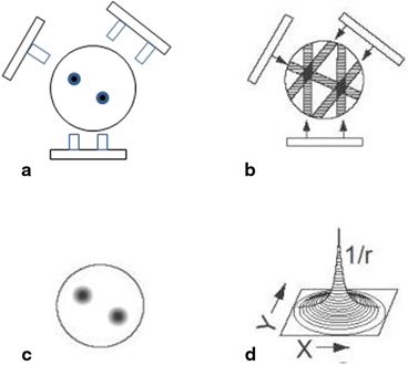
Fig. 12.3

Basic principle of reconstruction of an image by the backprojection technique. a An object with two “hot” spots (solid spheres) is viewed at three projections (at 120° angles). Each pixel count in a projection represents the sum of all counts along the straight-line path through the depth of the object. b Collected data are used to reconstruct the image by backprojection. c When many views are obtained, the reconstructed image represents the activity distribution with “hot” spots. d Blurring effect described by 1/r function where r is the distance away from the central point

Backprojection can be better explained in terms of data acquisition in the computer matrix. Suppose the data are collected in a 4 ´ 4 acquisition matrix, as shown in Fig. 12.4a. In this matrix, each row represents a slice, projection, or profile of a certain thickness and is backprojected individually. Each row consists of four pixels. For example, the first row has pixels A₁, B₁, C₁, and D₁. Counts in each pixel are considered to be the sum of all counts along the depth of the view. In the backprojection technique, a new reconstruction matrix of the same size (i.e., 4 ´ 4) is designed so that counts in pixel A₁ of the acquisition matrix are added to each pixel of the first column of the reconstruction matrix (Fig. 12.4b). Similarly, counts from pixels B₁, C₁, and D₁ are added to each pixel of the second, third, and fourth columns of the reconstruction matrix, respectively.

Fig. 12.4

An illustration of the backprojection technique using the data from an acquisition matrix into a reconstruction matrix

Next, suppose a lateral view (90°) of the same object is taken, and the data are again stored in a 4 ´ 4 acquisition matrix. The first row of pixels (A₂, B₂, C₂, and D₂) in the 90° acquisition matrix is shown in Fig. 12.4c. Counts from pixel A₂ are added to each pixel of the first row of the same reconstruction matrix, counts from pixel B₂ to the second row, counts from pixel C₂ to the third row, and so on. If more views are taken at angles between 0 and 90°, or any other angle greater than 90° and stored in 4 ´ 4 acquisition matrices, then the first row data of all these views can be similarly backprojected into the reconstruction matrix. This type of back-projection results in superimposition of data in each projection, thereby forming the final transverse image with areas of increased or decreased activity (Fig. 12.3c).

Similarly, backprojecting data from the other three rows of the 4 × 4 matrix of all views, four transverse cross-sectional images (slices) can be produced. Therefore, using 64 × 64 matrices for both acquisition and reconstruction, 64 transverse slices can be generated. From transverse slices, appropriate pixels are sorted out along the horizontal and vertical long axes, and used to form sagittal and coronal images, respectively. It is a common practice to lump several slices together to increase the count density in the individual slices to reduce statistical fluctuations.

Filtered Backprojection

The simple backprojection has the problem of “star pattern” artifacts (Fig. 12.3c) caused by “shining through” radiations from adjacent areas of increased radioactivity resulting in the blurring of the object . Because the blurring effect decreases with distance (r) from the object of interest, it can be described by a 1/r function (Fig. 12.3d). It can be considered as a spillover of certain counts from a pixel of interest into neighboring pixels, and the spillover decreases from the nearest pixels to the farthest pixels. This blurring effect is minimized by applying a “filter” to the acquisition data, and the filtered projections are then backprojected to produce an image that is more representative of the original object. Such methods are called the filtered backprojection . There are in general two methods of filtered backprojection: the convolution method in the spatial domain and the Fourier method in the frequency domain , both of which are described below.

The Convolution Method

The blurring of reconstructed images caused by simple backprojection is eliminated by the convolution method in which a function, termed “kernel,” is convolved with the projection data, and the resultant data are then backprojected. The application of a kernel is a mathematical operation that essentially removes the l/r function by taking some counts from the neighboring pixels and putting them back into the central pixel of interest. Mathematically, a convolved image f′(x, y) can be expressed as

${f}'(x,\text{ }y)=\sum\limits_{i=-N}^{N}{\sum\limits_{j=-N}^{N}\!\!{{{h}_\textit{ij}}}}\odot {{f}_\textit{ij}}(x-i,\;y-j)$

(12.1)

where f _ij(x − i, y − j) is the pixel count density at the x − i, y − j location in the acquired projection, the h _ijvalues are the weighting factors of the convolution kernel, and ⊙ indicates the convolution operation. The arrangement of h _ijis available in many forms.

A familiar “nine-point smoothing” kernel (i.e., 3 × 3 size), also called smoothing filter, has been widely used in nuclear medicine to decrease statistical variation. The essence of this technique is primarily to average the counts in each pixel with those of the neighboring pixels in the acquisition matrix. An example of the application of nine-point smoothing to a section of an image is given in Fig. 12.5. Let us assume that the thick-lined pixel with value 5 in the acquisition matrix is to be smoothed. First, we assume a 3 × 3 acquisition matrix (same as 3 × 3 kernel matrix) centered at the pixel to be convolved. Each pixel datum of this matrix is multiplied by the corresponding weighting factor, followed by the summation of the products. The weighting factors are calculated by dividing the individual pixel values of the kernel matrix by the sum of all pixel values of the matrix. The result of this operation is that the value of the pixel has changed from 5 to 3. Similarly, all pixels in the acquisition matrix are smoothed, and the profiles are then backprojected.

Fig. 12.5

The smoothing technique in the spatial domain using a 9-point smoothing kernel. The thick-lined pixel with value 5 is smoothed by first assuming a 3 × 3 acquisition matrix (same size as the smoothing matrix) centered at this pixel and multiplying each pixel value of the matrix by the corresponding weighting factor, followed by summing the products. The weighting factor is calculated by dividing the individual pixel value by the sum of all pixel values of the smoothing matrix. After smoothing the value of the pixel is changed from 5 to 3. Similarly all pixel values of the acquisition matrix are smoothed by the nine-point smoothing kernel, to give a smoothed image

The spatial kernel described above with all positive weighting factors reduces noise but degrades spatial resolution of the image. Sharp edges in the original image become blurred in the smoothed image as a result of averaging the counts of the edge pixels with those of the neighboring pixels.

Another filter kernel commonly used in the spatial domain consists of a narrow central peak with both positive and negative values on both sides of the peak, as shown in Fig. 12.6. When this so-called edge-sharpening filter is applied centrally to a pixel for correction, the negative values in effect cancel or erase all neighboring pixel count densities, thus creating a corrected central pixel value. This is repeated for all pixels in each projection and the corrected projections are then backprojected. This technique reproduces the original image with better spatial resolution but with increasing noise. Note that blurring due to simple backprojection is removed by this technique but the noise inherent in the data acquisition due to the limitations of the spatial resolution of the imaging device is not removed but rather enhanced.

Fig. 12.6

A filter in the spatial domain. The negative side-lobes in the spatial domain cancel out the unwanted contributions that lead to blurring in the reconstructed image

The Fourier Method

Nuclear medicine data obtained in the spatial domain (Fig. 12.7a) can be expressed in terms of a Fourier series in the frequency domain as the sum of a series of sinusoidal waves of different amplitudes, spatial frequencies, and phase shifts running across the image (Fig. 12.7b). This is equivalent to sound waves that are composed of many sound frequencies. Thus, the data for each row and column of the acquisition matrix can be considered as composed of sinusoidal waves of varying amplitudes and frequencies in the frequency domain. The process of determining the amplitudes of sinusoidal waves is called the Fourier transformation (Fig. 12.7c) and the method of changing from the frequency domain to the spatial domain is called the inverse Fourier transformation.

Fig. 12.7

Representation of an object in the spatial and frequency domains. A profile in the spatial domain can be expressed as an infinite sum of sinusoidal functions (the Fourier series). For example, the activity distribution as function of distance in an organ (a) can be composed by the sum of the four sine functions (b). The Fourier transform of this activity distribution is represented in (c), in which the amplitude of each sine wave is plotted at the corresponding frequency of the sine wave

The Fourier method of reconstruction can be applied in two ways: either directly or by using filters. In the direct Fourier method, the Fourier transforms of individual acquisition projections are taken in polar coordinates in the frequency domain , which are then used to calculate the values in rectangular coordinates. Inverse Fourier transforms of these profiles are taken to compute the image. The method is not a true backprojection and is rarely used in reconstruction of images in nuclear medicine because of the time-consuming computation.

A more convenient method of reconstruction is the filtered backprojection (FBP) using the Fourier technique. In this method, filters are used to eliminate the blurring function l/r that arises from simple backprojection of the projection data. These filters are analogous to tone controls or equalizers in radios or CD players that act as filters to vary the amplitudes of different frequencies, bass for low-frequency amplitudes and treble for high-frequency amplitudes. In image reconstruction, filters do the same thing, modulating the amplitudes of different frequencies, preserving the broad structures (the image) represented by low frequencies and removing the fine structures (noise) represented by high frequencies.

The Fourier method of filtering the projection data is based on the initial transformation of these data from the spatial domain to the frequency domain, which is symbolically expressed as

${\rm F}({{v}_{x}},{{v}_{y}})={\cal {F}}{f}(x,y)$

(12.2)

where F(ν _x, ν _y) is the Fourier transform of f(x, y) and Ƒ denotes the Fourier transformation. Next a Fourier filter, H(ν) is applied in the frequency domain; that is,

${\rm F}'(v)={\rm H}(v)\cdot {\rm F}(v)$

(12.3)

where F′(ν) is the filtered projection in the frequency domain, which is obtained as the multiplication product of H(ν) and F(ν). Finally, the inverse Fourier transformation is performed to obtain the filtered projections, which are then backprojected. The results obtained by the Fourier method are identical to those obtained by the convolution method. Although the Fourier method appears to be somewhat cumbersome and difficult to understand, the use of modern computers has made it much easier and faster to compute the reconstruction of images than the convolution method .

Types of Filters

A number of Fourier filters have been designed and used in the reconstruction of images in nuclear medicine. All of them are characterized by a maximum frequency, called the Nyquist frequency, that gives an upper limit to the number of frequencies necessary to describe the sine or cosine curves representing an image projection. Because the acquisition data are discrete, the maximum number of peaks possible in a projection would be in a situation in which peaks and valleys occur in every alternate pixel (i.e., one cycle per two pixels or 0.5 cycle/pixel), which is the Nyquist frequency. If the pixel size is known for a given matrix, then the Nyquist frequency can be determined. For example, if the pixel size in a 64 × 64 matrix is 4.5 mm for a given detector, then the Nyquist frequency will be

$\begin{aligned} \text{Nyquist frequency}&=0.5\; \text{cycle/pixel} \nonumber\\ & = 0.5\; \text{cycle/0.45 cm}\nonumber\\ & = 1.11\; \text{cycles/cm}\end{aligned}$

A common and well-known filter is the ramp filter (name derived from its shape in the frequency domain) shown in Fig. 12.8 in the frequency domain. An undesirable characteristic of the ramp filter is that it amplifies the noise associated with high frequencies in the image even though it removes the blurring effect of simple backprojection. To eliminate the high-frequency noise, a window is applied to the ramp filter. A window is a function that is designed to eliminate high-frequency noises and retain the low-frequency patient data. Typical filters that are commonly used in reconstruction are basically the products of a ramp filter that has a sharp cut-off at the Nyquist frequency (0.5 cycle/pixel) and a window with amplitude 1.0 at low frequencies but gradually decreasing at higher frequencies. A few of these windows (named after those who introduced them) are illustrated in Fig. 12.9, and the corresponding filters (more correctly, filter–window combinations) are shown in Fig. 12.10.

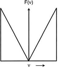
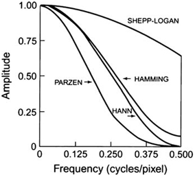
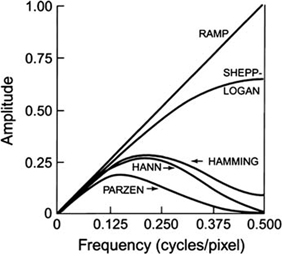
Fig. 12.8

The ramp filter in the frequency domain

Fig. 12.9

Different windows for reconstruction filters in SPECT. Different windows suppress the higher spatial frequencies to a variable degree with a cutoff Nyquist frequency of 0.5 cycle/pixel

Fig. 12.10

Different filters for SPECT that are obtained by multiplying the respective windows by the ramp filter with cutoff at Nyquist frequency of 0.5 cycle/pixel

The effect of a decreasing window at higher frequencies is to eliminate the noise associated with them. The frequency above which the noise is eliminated is called the cut-off frequency. As the cut-off frequency is increased, spatial resolution improves and more image detail can be seen up to a certain frequency. At a too high cut-off value, image detail may be lost due to inclusion of inherent noise. Thus, a filter with an appropriate cut-off value should be chosen so that primarily noise is removed, and image detail is preserved. Note that the Nyquist frequency is the highest cut-off frequency for a reconstruction filter and typical cut-off frequencies vary from 0.2 to 1.0 times the Nyquist frequency. Filters are selected based on the amplitude and frequency of noise in the data. Normally, a filter with a lower cut-off value is chosen for noisier data as in the case of obese patients and in ²⁰¹Tl myocardial perfusion studies or other studies with poor count density.

Hann, Hamming, Parzen, and Shepp–Logan filters are all low-pass filters because they preserve low-frequency structures, while eliminating high-frequency noise. All of them are defined by a fixed formula with a user-selected cut-off frequency. It is clear from Fig. 12.10 that most smoothing is provided by the Parzen filter and the Shepp–Logan filter produces the least smoothing.

An important low-pass filter that is most commonly used in nuclear medicine is the Butterworth filter (Fig. 12.11). This filter has two parameters: the critical frequency (v _c) and the order or power (n). The critical frequency is the frequency at which the filter attenuates the amplitude by 0.707, but not the frequency at which it is reduced to zero as with other filters. The parameter, order or power n, determines how rapidly the attenuation of amplitudes occurs with increasing frequencies. The higher the order, the sharper the fall. Lowering the critical frequency, while maintaining the order, results in more smoothing of the image.

Fig. 12.11

Butterworth filter with different orders and cutoff frequencies

Another class of filters, the Weiner and Metz filters, enhances a specific frequency response.

Many commercial software packages are available offering a variety of choices for filters and cut-off values. The selection of a cut-off value is important such that noise is reduced and image detail is preserved. Reducing a cut-off value will increase smoothing but will curtail low-frequency patient data and thus degrade image contrast particularly in smaller lesions. No filter is perfect and, therefore, the design, acceptance, and implementation of a filter are normally done by trial and error with the ultimate result of clinical utility.

As already mentioned, filtered backprojection was originally applied only to transverse slices from which vertical and horizontal long axis slices are constructed. Filtering between the adjacent slices is not performed, and this results in distortion of the image in planes other than the transverse plane. With algorithms available in current SPECT systems, filtering can be applied to slices perpendicular to transverse planes or in any plane through the 3-D volume of an object. This process is called volume smoothing. However, because of increased popularity of iterative methods described below, the 3-D volume smoothing is not widely applied.

Iterative Reconstruction

The basic principle of iterative reconstruction involves a comparison between the measured image and an estimated image that is repeated until a satisfactory agreement is achieved . In practice, an initial estimate is made of individual pixels in a projection of a reconstruction matrix of the same size as that of the acquisition matrix, and the projection is then compared with that of the measured image. If the estimated pixel values in the projection differ from the measured values, a correction is calculated from the ratio or difference between the two values for each projection, which is applied to each pixel in the projection to obtain an updated estimated projection for the next comparison with the measured projection. This process is repeated until a satisfactory agreement is obtained between the estimated and actual images. The schematic concept of iterative reconstruction is illustrated in Fig. 12.12. The method makes many iterations requiring long computation time and with the availability of faster computers nowadays, the method is routinely used in image reconstruction in PET , SPECT , CT and MR imaging.

Fig. 12.12

Conceptual scheme of iterative reconstruction

Consider a radioactive source of 5 × 5 pixel cross-sectional matrix containing varied amount of activity in each pixel as illustrated in Fig. 12.13a. Only three measured projections A, B, and C obtained at different angles are shown with five bins each, which are basically the pixels in a row of the acquisition matrix in line with the source matrix. Since all pixels do not contribute equally, a weighted sum of the contributions from each pixel makes up the measured activity p _iin the ith bin, that is,

Fig. 12.13

a Three projections A, B, and C each with 5 bins taken of a 5 × 5 cross-sectional matrix. Counts p _iis the weighted sum of counts contributed by each pixel in a row of acquisition matrix, as given by Eq. (12.4). b Concept of weighting factor, a _ij

${{p}_{i}}=\sum\nolimits_{j=1}^{m}{{{a}_{\textit{ij}}}\;{{q}_{j}}}$

(12.4)

where q _jis the counts (activity) in the jth pixel and a _ijis the probability that an emission from pixel j is recorded in the ith bin. The concept of a _ijis illustrated in Fig. 12.13b, which is given by the shaded area of the pixel j along the ith bin.

Only gold members can continue reading. Log In or Register to continue