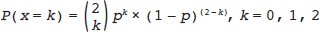
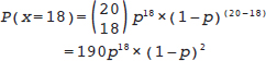
13 • To explain point estimation. • To describe interval estimation and confidence intervals. • To describe the logic of hypothesis testing. • To present methods of analysis of some common study designs. The previous chapter on exploratory data analysis and descriptive statistics (Chapter 2) covered methods for using an observed sample of data to describe and explore its most interesting features. However, we do not usually want to restrict our conclusions to the particular sample that we took, but instead, we want to use that data to make more general statements about relationships in the broader population. For example, if we take a sample of 20 patients with known liver malignancies and find that 18 of them had abnormal ultrasound findings in the month before their biopsy, what is the reason that we use 18/20 = 90% as the estimate of the detection percentage for ultrasound in the population of patients with liver malignancies? Given this estimated value of 90%, what are the smallest and largest plausible values for the detection percentage in the larger population? How sure are we that the actual percentage in all patients was not 60% and we got “lucky” with this sample? This chapter explains the statistical methods for answering these questions. To move beyond simple descriptive statistics, and to use a sample to make inferences about the population, we need to consider two key elements: (1) the statistical model which is presumed to have generated the observed data; and (2) the manner in which the sample was taken.1,2 The first element is the focus of this chapter; the second element, selection of the sample, is crucial to analysis of data and can have an influence on how generalizable the results of an analysis are to the wider population (see Chapter 5), but is not considered in any detail here. A statistical model is a construction that links unobserved (and unobservable) quantities in the population to the observed data. We will illustrate by constructing a model for the example introduced above, where the observed data are the abnormal ultrasounds in patients with liver malignancies and the unobserved quantity is the true detection percentage. First, we define the population as all patients with liver malignancies who have an ultra-sound in the month before a definitive biopsy. Then, we introduce the idea of a probability, in this case the fraction of the population that has an abnormal ultrasound in the month before their biopsy. In statistics, this probability is usually represented by the letter p. To simplify the wording, we will refer to an abnormal ultrasound as an “event.” Finally, we have the notion of a sample, the number of patients (in this example) taken from the larger population and assessed. If we randomly sample one patient from the entire population, what is the probability that this patient will have an event? By definition, it is p and the probability of the patient not having an event is 1 – p. But what if we randomly sample two patients? Given that we observe a sample on two patients, what is the probability that we observe zero events on these two patients? One event? Two events? When the outcomes on the two patients are independent, we multiply the probability of the outcome on one patient by the probability of the outcome on the second patient to obtain the total probability for the two patients. So that we do not have to keep repeating the phrase “the number of events,” we use x to represent this idea. The probability that x = 2 is found by multiplying the probability that the first patient has an event times the probability that the second patient does: Similarly, the probability that neither patient has an event (so that x = 0) is There are two equally likely combinations of outcomes that give x = 1: the first patient has an event and the second does not; the first patient does not have an event but the second does. We need to add probabilities for both combinations to get the probability that x = 1: These equations can be expressed as a single equation that gives the probability of observing k = 0, 1, or 2 events in a sample size of 2. The notation If we now replace 2 with any value of n, we have an equation that defines what is called the binomial model. It computes the probability of observing k events in n subjects, when each subject has the same probability p of having an event: How does all of this mathematics help us estimate the true value of p from sample data? The model provides the link between the data (e.g., 18/20) and the quantity we are interested in (p, the probability of an abnormal ultrasound). Filling in k A widely used method, maximum likelihood, uses this equation to find the value of p that makes the observed value of 18 most likely; in other words, it finds p at the maximum of the curve in Fig. 13.1, a plot of p(x = 18) versus values of p between 0.6 and 1. Among all possible values of p, it is the value 0.9 that makes the observed 18 events in 20 patients most likely and this is what we use as an estimate, Fig. 13.1 also shows us something else important—there are some values of p that are almost as good as 0.9 (e.g., 0.85) but there are some values (e.g., p Fig. 13.2 shows the probability of each possible number of abnormal ultrasounds if the true probability of any one being abnormal is 0.7. These correspond to estimated Suppose that the data in our example were collected in a radiology department that was attempting to achieve a detection percentage above 70%. With 18 abnormalities detected in 20 patients, can we conclude that this target is being met? To answer this question, we can set up two competing hypotheses, called the null (H0) and alternative (Ha). H0: p < 0.70 [The department is not meeting its goals] Ha: p ≥ 0.70 [The department is meeting its goals] We start by noting that if we decided the target was met based on 18 events in 20 patients, we would also have made that same decision if we had seen 19 or 20 events on these 20 patients. If 18 is a large enough number that we conclude p There is only a 3.6% probability of observing such high numbers (18, 19, or 20) if the detection rate is an unacceptable 70%. The bars for 18, 19, and 20 abnormalities, shaded red in Fig. 13.2, have a total probability of 3.6%. This number is called the p value for a test of the hypothesis that the detection rate was 0.7 or less. But what should be done with the p value? Does the radiology department decide that detection rates are not unacceptably low? The p value was introduced by the statistician R.A. Fisher as a measure of evidence against the null hypothesis: the smaller the p value, the less likely the observed data under the null hypothesis and, therefore, the stronger the evidence against that null hypothesis. Notably, Fisher did not suggest that the p value alone should be used to interpret the evidence but believed that it was one piece of a process that also took into account background information.3,4 According to this view, the p value of 0.036 has to be interpreted by the investigator in light of other pertinent information. A 2016 consensus statement issued by the American Statistical Association, the primary American professional association for statisticians, emphasized this view, stating “Scientific conclusions and business or policy decisions should not be based only on whether a p-value passes a specific threshold.”5 Hypothesis testing plays a central role in analyses of data from medical research, so we expand here on the logic of this approach. In general, there are four important elements to a statistical test: 1. The null hypothesis (H0) 2. The alternative hypothesis (Ha) 3. The test statistic 4. The rejection region or the threshold value for rejecting H0 Let’s return to our ultrasound detection rate example, where the head of radiology needs to make a decision as to whether the detection percentage is above or below 70%. We formulate our statistical hypothesis testing problem as: The test statistic in this example is the number of the 20 cases that are detected. We use this statistic to decide whether to reject H0. The rejection region will be a prespecified set of values (e.g., 15 or more; or 18 or more) that will lead us to reject the null hypothesis. The magnitude our test statistic forces us to make a binary decision as to whether or not we are in the rejection region, once we have observed the study data. The pairing of the null and alternative hypotheses with the decision to reject the null hypothesis or not reject it means that there are four possible outcomes of a hypothesis test. These are shown in Table 13.1 where, to make matters concrete, we have set the rejection region to be either 19 or 20 abnormal ultrasounds. Table 13.1 Outcomes of hypothesis testing
Statistical Inference: Point Estimation, Confidence Intervals, and Hypothesis Testing
 Learning Objectives
 Introduction
 Example of a Statistical Model
P(x = 2) = p × p = p2
P(x = 0) = (1 – p) × (1 – p) = (1 – p)2
P(x=1)=p×(1–p) + (1–p)×p=2×p×(1–p)
 is read as “2 choose k” and says how many different ways there are to pick k items from a set of 2.

Estimating p
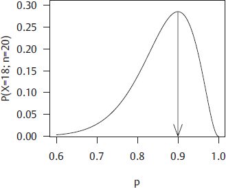
= 18 and n = 20, Equation 1 has only one unknown, p:
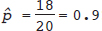 ; the “hat” or circumflex in
 ^p (“p hat”) indicates that it is not the true value (which we cannot know) but an estimate of it. It is possible to use calculus to find the value of p at the maximum of the curve in Fig. 13.1, but we don’t need to. The estimator in the binomial model is always  .
.
Estimating a Confidence Interval for p
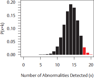
= 0.6) that have much less support from the data. Maximum likelihood theory provides a way to use the observed data (18 out of 20) and the model (binomial) to obtain a range of values for p—an interval—that has some degree of plausibility and to exclude from this interval values that are implausible. Most commonly, this interval is constructed to have 95% “confidence.” The technical definition of the 95% confidence interval is rather wordy: a confidence interval has 95% coverage if in 95% of repeated random samples from the same population, the interval that is constructed includes the true (unknown) value. Our advice is to remember this definition but to think of the 95% confidence interval as a range of values that is very likely to include the true value. With 18 events in 20 patients; one approach to construction of a 95% confidence interval gives [0.72, 0.98]. Values for p outside this range are less likely than values in it, and we have 95% confidence that this interval covers the true value.
Sampling Variability
 values of 0/20, 1/20, 2/20,…, 20/20. Our estimator x/n has what is called a sampling distribution; if we know p, we know the probability of getting each value
  . The variability of
  around its expected value of 0.7 can be measured by a quantity called the standard error. For the binomial model, the standard error is equal to
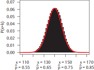
 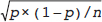 . Fig. 13.3 shows the results of the same experiment run on a larger sample of n = 200, again assuming that the true percentage abnormal is 0.7; here, the standard error is
  . Many estimators presented later in this chapter share a property of the estimate of the binomial probability: in repeated samples from the same population, they will approximately have what is called a normal distribution with a mean equal to the true value and variability about that mean equal to the standard error.
Hypothesis Testing
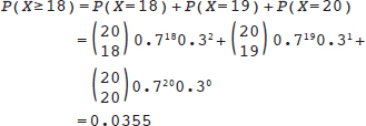
> 0.70, then clearly 19 and 20 are also high enough. Thus, we can phrase the question as, “If the department is not meeting its goals, what is the chance of seeing ultrasound performance at least as good as I have observed?” or “If the true detection percentage is 70%, what is the probability that I will observe 18, 19, or 20 detected abnormalities in a sample of 20 patients?” Our statistical model (i.e., the binomial probability model) provides the answer to that question. If we assume that the true value of p is as low as 0.7, we can calculate the chance of observing values as high as we did through this formula:

Decision | (Unknown) Truth |
|
| Null hypothesis true p ≤ 0.70 | Null hypothesis false p > 0.70 |
x = 19 or x = 20 → Reject H0 | Type 1 error | Correct rejection of null hypothesis |
x ≤ 18 → Fail to Reject H0 | Correct nonrejection of null hypothesis | Type 2 error |
We observed x = 18, so with our rejection region, we will not reject H0. We are not able to reject the hypothesis of a low true detection rate. Importantly, we do not accept the null hypothesis and decide that the detection percentage is below 70%; that would be bizarre, given that we observed a detection percentage of 90%. The conclusion is that the count was not high enough to rule out a true value of 70%. We are in the second row of Table 13.1, where we are either correct to not reject H0 (column 1) or we are incorrect (column 2); we don’t know which column we are in, because we don’t know whether the null hypothesis is true or not. But if in fact the null hypothesis is false, when we do not reject it, we commit what is called a type 2 error.
Now let’s assume that the head of radiology demands a second study assessing the liver abnormality detection percentage on ultrasound. In this second study, analyzed according to the same rules as detailed in Table 13.1, 19 of 20 cases with liver malignancies had an abnormal ultrasound. In this second study, we reject the null hypothesis, so we are situated in the first row of Table 13.1 and we are either correct to reject H0 (column 2) or we are incorrect (column 1). If in fact the null hypothesis is true, when we reject it we commit what is called a type 1 error.
Suppose that the true detection percentage is 70% and we set the rejection region at 18 or more cases in a sample of 20; we can use the equation defining the binomial probability model to show that there is a probability of 0.0355 that we will obtain 18 or more abnormal ultrasounds. If we had set the rejection region at 19 or more cases, then from the equation defining the binomial probability model, we see that there is a probability of 0.0076 of observing data in the rejection region. By picking a rejection region before we carry out the study (e.g., 18 or more abnormal ultrasounds), we control the chance of making a type 1 error. Conventionally, rejection regions are set up to keep the type 1 error probability at 5% or lower. This way, when a null hypothesis is true, we will reject it in no more than 5% of studies. One way to keep the type 1 error rate below 5% is to reject the null hypothesis when a p value is < 0.05.
Outline of Remaining Parts of Chapter
In the remainder of this chapter, we illustrate how to analyze and interpret data arising from common research designs, with commonly encountered research questions. We will start with analysis of binary variables and then show the methods for similar designs analyzing continuous variables. All analyses will use a dataset on cartilage degeneration that has 40 individuals each measured at a baseline (time 1) and a follow-up time point (time 2). There are several baseline patient characteristics that do not change over time:
• Age at enrollment (years)
• Sex (male/female)
• Ethnicity (Caucasian/African-American/other)
The outcome is the extent of cartilage degeneration in the knee joint and it is measured at both the baseline and follow-up time points. It is measured in three ways:
• Continuous: area of degeneration in mm2
• Binary: cartilage degeneration vs. no cartilage degeneration
• Ordinal: degeneration graded as limited (0–2), mild (2–4), moderate (4–6), or severe (>6)
• Nominal: cartilage degeneration level (structural, functional, molecular)
The dataset and R code for conducting these analyses can be found on the companion web-site in the materials for this chapter.
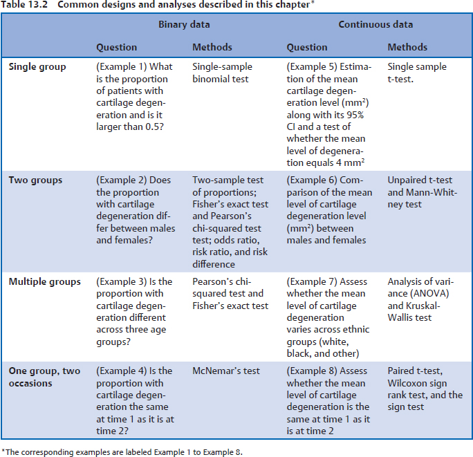
The statistical methods used in the remainder of this chapter are shown in Table 13.2, where they are categorized by the type of outcome and the type of question being asked. The concepts for each of the examples in Table 13.2 will be discussed as they are encountered and we will also show how to carry out each of these analyses using the R programming language.
 Common Study Designs and Analyses
Example 1: One Group with Binary Data
We are interested in the underlying probability of cartilage degeneration, based on a sample of patients who have been classified as having degeneration or not. In this example, we illustrate how to:
• Estimate the proportion of cases with cartilage degeneration
• Construct a 95% confidence interval for this proportion
• Test whether this proportion is equal to 0.5
Let n be the number of patients in the sample and X be the number with mild to severe degeneration. We estimate the sample proportion as follows:


