Chapter 14 The AC transformer
Chapter contents
14.1 Aim
The aim of this chapter is to discuss the main concepts that govern the operation of the step-up or the step-down alternating current (AC) transformer. In addition to this, two forms of specialist transformers are discussed, namely the autotransformer and the constant-voltage transformer. Finally, there is an overview of the factors that affect transformer rating and how these factors relate to radiographic exposures.
14.3 The ideal transformer
Let us start by defining this device:
Consider such an ideal transformer, shown in Figure 14.1, where two isolated sets of windings share a common core – there are a number of other configurations of core and windings but the one shown in Figure 14.1 is the simplest. The input or primary side of the transformer consists of np turns around the core and has an alternating voltage VP across it. The output or secondary side of the transformer consists of ns turns and has a voltage Vs induced in it. This is a case of mutual induction, as discussed in Section 10.7. The sequence of events is as follows:
• The alternating voltage in the primary winding VP causes an AC to flow through the winding.
• This AC, Ip, produces a changing magnetic flux density (B) in the soft iron core.
• The changing magnetic flux density is linked to the secondary winding so that an electromotive force (EMF), Vs, is induced in it according to Faraday’s and Lenz’s laws of electromagnetic induction (see Sects 10.4 and 10.5).
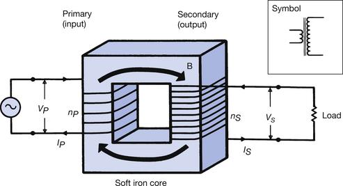
Figure 14.1 An ‘ideal’ transformer showing the core and the primary and secondary windings. In practice, the core is laminated, as shown in Figure 14.2. As there are more turns on the secondary winding than on the primary winding, this is a step-up transformer. The symbol for a step-up transformer is also shown. See text for details.
The purpose of the soft iron core is to contain all the magnetic flux within it so that the magnetic flux linkage between the primary and the secondary is as near perfect as possible. The core is able to do this because of its strong induced magnetism, resulting from its high magnetic permeability (see Table 14.1).
Table 14.1 A summary of the losses associated with a particular transformer
| TRANSFORMER LOSS | COMMENTS |
|---|---|
| Copper losses | Caused by the resistance of the copper windings. Also known as I2R losses |
| Iron losses | Losses produced in the transformer core |
| Imperfect magnetic flux linkage | Very small loss flux |
| Eddy currents | Caused by electromagnetic induction within the core of the transformer – reduced by core lamination |
| Hysteresis | Caused by the work required to move the magnetic domains – reduced by the appropriate choice of core material (e.g. stalloy) |
| Regulation (a consequence of all the above losses) | Output voltage decreases with increased current load because of the increased losses due to the resistance of the windings |
The mathematics of the ideal transformer are relatively simple if we first consider the effect of the magnetic flux on a single turn of wire around the core. Since we are assuming that the transformer is ideal, there is no magnetic flux loss and the EMF induced is independent of the position of the wire. Thus, the same voltage will be induced in each turn of the primary and in each turn of the secondary. If we call this voltage v, then we can say that the total primary voltage is the voltage in each turn multiplied by the number of turns. Thus:


Thus, we can combine the two equations above to get:

By cross-multiplying this equation, we get the formula:


From Equation 14.1 we know:

Thus, for an ideal transformer, we can say:

14.4 Faraday’s laws and lenz’s law applied to transformers
We have already considered Faraday’s laws of electromagnetic induction (Sect. 10.4) and Lenz’s law (Sect. 10.5) and we can now look at how these are applied to transformers.