The Early Days of Modeling Contrast Agent Kinetics
Paul S. Tofts
Dynamic Contrast-Enhanced MRI: The Stimulus to Model Multiple Sclerosis Data
In 1985, I was appointed as a “new blood” lecturer at the Institute of Neurology, Queen Square, London, in the multiple sclerosis (MS) research group headed by the late Ian McDonald, the leading MS clinician in the United Kingdom at the time. A physicist by training, with a PhD in nuclear magnetic resonance of solid helium at low temperatures, I was thrown into a clinical research environment, with the brief to develop the newly installed nuclear magnetic resonance imaging (MRI) technology. My passion had always been to use physics to contribute to human health, so this suited me perfectly. The UK Multiple Sclerosis Society had in the previous year funded a 0.3T Picker MRI machine, and a whole range of techniques to study the biology of developing MS lesions was being developed.
In the next few years, Schering AG, a company based in Berlin, produced the first MRI contrast agent (then called gadolinium-diethylene triamine pentaacetic acid [Gd-DTPA], now Magnevist), and Queen Square was one of the first centers to use it for MS imaging. Previous work at Hammersmith Hospital by Ian Young and colleagues had shown that MS lesions, having a defective blood–brain barrier (BBB), would enhance after injection of the compound.
Allan Kermode was a curious and dynamic trainee neurologist, the son of an Australian surgeon in Perth; he asked me how long after injection of the contrast agent should he image to stand the best chance of seeing image signal enhancement. This provoked a creative discussion in which I suggested trying a range of times to optimize the procedure. I thought no more about it, at the time being preoccupied with writing up previous work on quantification in spectroscopy.
A week later, Kermode came back to me with datasets from two patients showing very different enhancement patterns. In each he had measured the mean signal in a region of interest over periods of time up to nearly 2 hours (Fig. 83.1). This was many years before ethical considerations slowed down clinical research. The patients had come out of the scanner for a break during the long examination, and good manual repositioning by the radiographer (technologist) gave datasets in which the portions collected before and after the break were spatially registered. Imaging was slow (a single slice inversion recovery sequence gave data every 6 minutes or so, a lesson in patience compared with modern acquisition; see Chapter 23).
This provoked a firestorm in my brain; for weeks I could think of nothing else. What was driving this process? What biologic information was lurking beneath the image data? Weinmann et al.1 at Schering had measured the arterial plasma concentration of Gd-DTPA using blood samples every 5 minutes or so, and these were fitted to a biexponential model. The notion of water compartments had been revealed to me as part of my exposure to technetium (Tc99m) imaging at Hammersmith Hospital. I realized that the flow of gadolinium from the plasma through the leak in the endothelium to the extravascular space was governed by a mathematical differential equation, and this related to permeability as measured for many years in semipermeable membranes by physiologists. Solving differential equations had been part of my physics training at Oxford University. Finally, in a eureka moment, during a day working at home, at a place high on the roof terrace of my attic apartment that I still remember, it all fell into place. It became clear how to model the signal enhancement as a function of time (Fig. 83.2). (Much later on I became aware of the pharmacokinetic work already carried out by others.)
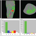
I rushed to the newly installed Sun Microsystems computer at Queen Square to set this up in Fortran (the programming language of the time). By altering the transfer constant (Ktrans) and the size of the extravascular extracellular space (ve) (Fig. 83.1), a set of model enhancement curves could be produced that really did have the behavior of the data that Kermode had given me. There was a peak in the enhancement, and the size and time of that peak could be changed by altering the two driving physiologic parameters: Ktrans and ve. By adjusting these, the two datasets could be fitted with no apparent systematic error. Programming in the least squares fitting gave an automated process where the curves would lie satisfyingly close to the data.
The value of Ktrans (at first called k, and in MS, equal to the permeability surface area product per unit volume of tissue) was reasonably close to values measured by physiologists in comparable tissues. The lowest observed value for the extracellular (interstitial) space volume fraction ve (21%) was a little more than the normal value (about 16%). In the slowly enhancing lesion, the value of 49% was considered implausibly high by the clinicians involved in experimental animal studies.
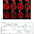
 FIGURE 83.1. (Left) Early dynamic contrast-enhanced data5 (A) rapidly enhancing multiple sclerosis lesion: Ktrans = 0.050 min−1, ve = 21%. (B) Slowly enhancing lesion: Ktrans = 0.013 min−1, ve = 49%. (Right) Model enhancement curves5 (A) fixed ve = 20%, varying Ktrans (K in the plot) showing how initial slope depends on Ktrans; (B) fixed Ktrans = 0.01 min−1, varying v(vi in the plot), showing how increased ve gives increased and delayed peak enhancement. |
The abstract by Kermode et al.2 at SMRM in 1988 prepared the way (see Geek Box 1). My poster at Los Angeles in February 1989 at the seventh annual meeting of the Society for Magnetic Resonance Imaging (SMRI; now part of the International Society of Magnetic Resonance in Medicine [ISMRM]) showed the essence of the method (Fig. 83.3).3 I did not personally attend; when Kermode returned from the meeting, he reported that he had met someone who was measuring T1 as a function of time after injection of Gd-DTPA in MS lesions, and that I had better publish my work quickly!
At the August meeting of the SMRM in Amsterdam in the same year, there were abstracts with remarkably similar titles from myself and Henrik Larsson, a Danish
clinician with a strong physiologic background. He was the mysterious person at SMRI that Kermode had told me about; we soon became friends. I proposed we write a joint note to reconcile the two approaches. Our own individual work4,5 was published (see Geek Box 2), then the reconciliation.6
clinician with a strong physiologic background. He was the mysterious person at SMRI that Kermode had told me about; we soon became friends. I proposed we write a joint note to reconcile the two approaches. Our own individual work4,5 was published (see Geek Box 2), then the reconciliation.6
 FIGURE 83.2. (Top) Compartment model used in original model5 (redrawn to use consensus31 names Ktrans and ve and explicit intravascular contribution vp). (Bottom) Key pharmacokinetic equations22: Ktrans and ve are defined in Figure 83.4; Cp, Ce, and Ct are the gadolinium concentrations in plasma, extravascular-extracellular space, and tissue. |
Geek Box 1
“Understanding the time course and degree of BBB (Blood-Brain Barrier) damage in plaques may give quantitative indices with which we can assess the efficacy of drugs aiming to correct BBB disturbances (e.g. steroids) and may prove to be of use in assessment of treatment in MS.”2
Histology studies showed that MS lesions could indeed have vast extracellular spaces (the “open lesions”). Modeling of transverse magnetization decay curves (where the signal from intracellular and extracellular water can be distinguished) showed that chronic lesions could have extracellular spaces up to 87% in MS,7 and that the large ve estimates from dynamic contrast-enhanced (DCE) MRI were indeed plausible (see Geek Box 3)! When asked what aspect of MRI physics I should concentrate on, Ian McDonald wisely pronounced: “well the quantitation seems rather interesting.”
Geek Box 2
“First we describe dynamic scanning, which enables a curve of signal enhancement versus time to be produced, with a consequent differentiation between lesions that enhance with different time courses. Second we describe a quantitative analysis of the dynamic curve which enables absolute measurements of blood-brain barrier permeability and leakage space to be made.”5
Quantification in MR: Absolute Metabolite Concentrations Using Spectroscopy
My first opportunity to quantify in biomedicine had been in the late 1970s using 31P spectra, before 1H MRI had begun. This was my first taste of how the application of quite specialized techniques from physics or mathematics could bring unexpected advances in biomedicine. A review was generously invited by John Griffiths, the editor of the newly formed journal NMR in Biomedicine; this appeared as its first article.8 The discovery that quantification using medical imaging is a fertile ground for innovation by physicists later inspired the first book on
quantification in MRI, focused on the brain9; recently a book on quantitative MRI in cancer has appeared.10
quantification in MRI, focused on the brain9; recently a book on quantitative MRI in cancer has appeared.10
 |
Geek Box 3
“When I started at Queen Square I was very junior. Perhaps being somewhat uninformed about existing dogma in MS was quite helpful in some ways and made me look at everything with a fresh view. John Prineas had seen large extracellular spaces in MS lesions; however everyone thought they were artefacts of the histology. The combination of dynamic MRI scanning with T2 decay studies (analysis into two compartments) changed forever the way pathologists thought about lesions. These lesions are the ‘black holes’ seen in T1-weighted imaging.”
Personal communication from Allan Kermode (2012). He reports his conversations with John Prineas, the principle MS pathologist at the time.
Early Pharmacokinetics by Physiologists: Teorell, Kety, and Patlak
Torsten Teorell has been called the father of pharmacokinetics.11 The papers from this physiologist at Uppsala University (Sweden) published in 1937 in a French journal on “The kinetics of distribution of substances administered to the body” are completely relevant to modern DCE modeling.12,13 He considers blood flow, blood volume, and permeability. Transport from the blood is described by a rate constant; differential equations are produced and solved (see Geek Box 4).11 The concepts of mass conservation (used by Fick the previous century) and differential equations (developed by Isaac Newton and others in the 17th century) naturally led to this work.
Related posts:
 Dose Considerations in CT Perfusion
 Confounding Effects in Arterial Spin Labeling
 Arterial Spin Labeling Acquisition Protocols
 Pediatric Stroke and Congenital Disease
 Clinical Applications of Dynamic Contrast-Enhanced Magnetic Resonance Imaging in Musculoskeletal Tumors
 Perfusion and Dynamic Contrast-Enhanced Imaging in White Matter Disease
Stay updated, free articles. Join our Telegram channel

Full access? Get Clinical Tree


