Ultrasound


Ultrasound


In ultrasound imaging, a short burst of mechanical energy created by a transducer is introduced into the body through contact with the skin. The resulting ultrasound pulse travels at the speed of sound in the tissues interacting with the many boundaries between organs and parenchyma and creating echoes from changes in the acoustic properties that return to the transducer receiver. Collection and recording of the echo amplitudes over time provide depth information about the tissues and echogenicity along the path of travel, which are encoded as grayscale values. Repeating the process hundreds of times with a small incremental change in the direction of the pulse produces a tomographic image of the insonated region (Fig. 14-1). In addition to two-dimensional (2D) tomographic imaging, ultrasound allows for anatomical distance and volume measurements, motion studies, blood velocity measurements, tissue stiffness measurements, and 3D imaging.

Imaging systems using ultrasound have attained a large presence in medical care within and outside of radiology and across many clinical domains, particularly in the past 10 years. The success of ultrasound is attributed to several characteristics, including the non-ionizing nature of ultrasound waves, the ability to produce realtime images of tissue structures in the body to deliver timely patient care, and the high portability and relatively low cost of Point of Care (PoC) systems. While handson training and practice are essential for the ultrasound practitioner, an understanding of the basic physics of ultrasound is central to the effective and safe use of this technology for medical imaging. This chapter describes the characteristics, properties, and production of ultrasound; interaction with tissues; instrumentation and equipment; image acquisition, processing, and display; achievable measurements including tissue stiffness and blood velocity; common artifacts; bioeffects; and safety considerations.


14.1 CHARACTERISTICS OF SOUND

Sound is mechanical energy that propagates through a continuous medium by the compression (high pressure) and rarefaction (low pressure) of particles that comprise it. Tissues can be considered to be elastic, like a spring. A mechanical inward deformation by an external force, such as a piston that pushes inward, causes a local increase in pressure and compression of the spring. As the piston moves backward during its cycle, a negative force causes a local decrease in pressure, causing the spring to elongate, while the compressed part of the spring moves forward with time, transferring the imparted energy to adjacent components (particles) of the spring. With constant motion of the piston, the energy continues to travel cyclically, as shown in the top diagram of Figure 14-2.


FIGURE 14-1 A major use of ultrasound is the acquisition and display of the acoustic properties of tissues. A transducer array (transmitter and receiver of ultrasound pulses) directs sound waves into the patient, receives the returning echoes, and converts the echo amplitudes into a 2D tomographic image using the ultrasound acquisition system. Exams requiring a high level of safety such as obstetrics are increasing the use of ultrasound in diagnostic radiology. (Photo credit: Emi Manning, UC Davis Health System.)
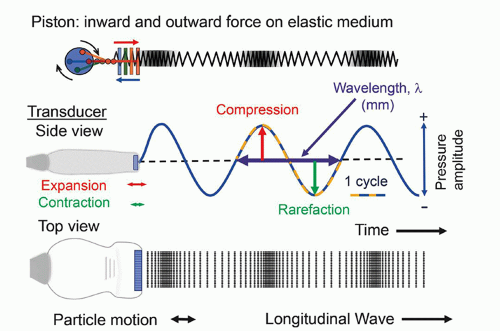
With ultrasound, the corresponding mechanical force is a transducer, made of an array of expanding and contracting crystal elements that form a surface area that is placed in contact with the tissues. During transducer surface expansion, an increase in the local pressure at the tissue surface occurs. Contraction follows, causing a decrease in pressure. The mechanical energy imparted at the surface is transferred to adjacent particles of the tissue, which travels at the speed of sound into the patient. Expansion and contraction of the transducer surface introduce energy into the medium as a series of compressions and rarefactions occurring every cycle, as shown in Figure 14-2 (middle diagram). A continuous tissue structure is necessary for mechanical energy transfer (i.e., sound propagation) as the constituent “particles” of the tissue act to transfer the mechanical energy with very small back-and-forth displacements. Energy propagation occurs as a wavefront in the direction of travel, known as a longitudinal wave, as shown in the bottom diagram of Figure 14-2.


FIGURE 14-2 Ultrasound energy is generated by mechanical displacement of an elastic medium, modeled as a compressible spring. An inward and outward force of a piston coupled to the medium creates increased pressure (compression) and decreased pressure (rarefaction) in a cyclical manner (top row). Constituents (particles) of the medium transfer energy to adjacent particles with minor back and forth displacement. The ultrasound transducer is the mechanical energy source that expands and contracts like the piston at very high frequency. This results in the introduction of ultrasound into the tissues, with propagation as a longitudinal wave. The wavelength is equal to the distance of one cycle.


14.1.1 Wavelength, Frequency, Speed

The wavelength (λ) is the distance between any two repeating points on the wave (a cycle) typically measured in millimeters (mm). The frequency (f) is the number of times the wave repeats per second (s), also defined in Hertz (Hz), where 1 Hz = 1 cycle/s. Frequency identifies the category of sound: less than 15 Hz is infrasound, 15 Hz to 20,000 Hz (20 kHz) is audible sound, and above 20 kHz, ultrasound. Medical ultrasound typically uses frequencies in the million (mega) cycles/s (MHz) range, from 1 to 20 MHz, with specialized ultrasound applications up to 50 MHz and beyond. The period is the time duration of one wave cycle and is equal to 1/f. The speed of sound, c, is the distance traveled per unit time through a medium and is equal to the wavelength (distance) divided by the period (time). As the frequency is equal to 1/period, the product of wavelength and frequency is equal to the speed of sound:


where c is the speed of sound, typically expressed in units of m/s, and often in cm/s and mm/µs. The speed of sound varies substantially within different materials, based on compressibility, stiffness, and density characteristics of the medium. The wave speed is determined by the ratio of the bulk modulus, B (a measure of the stiffness of a medium and its resistance to being compressed), and the density of the medium:


SI units are kg/(ms2), kg/m3, and m/s for B, ρ, and c, respectively. Sound propagates through a highly compressible medium such as air slowly, while sound propagates more rapidly through a less compressible medium such as bone. Soft tissues have compressibility and density characteristics with speeds as listed in Table 14-1. To relate time with propagation distance traveled in the patient, medical ultrasound devices assume a speed of sound of 1,540 m/s, despite slight differences in actual speed for the various tissues encountered. The speed of sound in soft tissue can be expressed in different units to simplify conversion factors or estimating values. The most common are 154,000 cm/s and 1.54 mm/µs.

Wavelength is the parameter that affects spatial resolution in an ultrasound image, with shorter wavelengths providing better spatial resolution. In a homogeneous medium or tissue, ultrasound frequency and speed of sound are constant; thus, a higher ultrasound frequency results in a shorter wavelength. Examples of the wavelength change as a function of frequency and propagation medium are given below.

EXAMPLE: A 2-MHz beam has a wavelength in soft tissue of (from Eq. 14-1):


A 10-MHz ultrasound beam has a corresponding wavelength in soft tissue of


Higher frequency sound has shorter wavelength, as shown in Figure 14-3.


TABLE 14-1 DENSITY, SPEED OF SOUND, AND ACOUSTIC IMPEDANCE FOR TISSUES AND MATERIALS RELEVANT TO MEDICAL ULTRASOUND
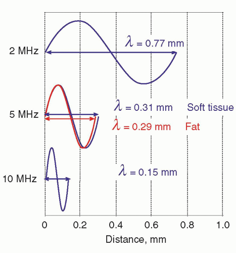


MATERIAL


DENSITY (kg/m3)


c (m/s)


Z (rayls)a


Air


1.2


330


3.96 × 10²


Lung


300


600


1.80 × 10³


Fat


924


1,450


1.34 × 10⁶


Water


1,000


1,480


1.48 × 10⁶


“Soft Tissue”


1,050


1,540


1.62 × 10⁶


Kidney


1,041


1,565


1.63 × 10⁶


Blood


1,058


1,560


1.65 × 10⁶


Liver


1,061


1,555


1.65 × 10⁶


Muscle


1,068


1,600


1.71 × 10⁶


Skull bone


1,912


4,080


7.8 × 10⁶


PZT


7,500


4,000


3.0 × 10⁷


a Acoustic impedance is the product of density and speed of sound. The named unit, rayl, has base units of kg/(m2s) for values listed in the column. Acoustic impedance directly relates to the propagation characteristics of ultrasound in each medium and is the basis for echo formation.


EXAMPLE: A 5-MHz beam travels from soft tissue into fat. Calculate the wavelength in each medium and determine the percent wavelength change.

In soft tissue,


In fat,


A decrease in wavelength of 5.8% occurs in going from soft tissue into fat, due to the differences in the speed of sound. This is depicted in Figure 14-3 for a 5-MHz ultrasound beam.


FIGURE 14-3 Ultrasound wavelength is determined by the frequency and the speed of sound in the propagation medium. Wavelengths in soft tissue are calculated for 2-, 5-, and 10-MHz ultrasound sources for soft tissue (blue). A comparison of wavelength in fat (red) to soft tissue at 5 MHz is also shown.


The wavelength in mm in soft tissue can be readily calculated by dividing the speed of sound in mm/µs (c = 1.54 mm/µs) by the frequency in MHz, as


Thus, the wavelength of a 10-MHz beam is easily determined as 1.54/10 = 0.154 mm, and that of a 2-MHz beam is 1.54/2 = 0.77 mm by using this simple change in units.

The spatial resolution of the ultrasound image and the attenuation of the ultrasound beam energy depend on the wavelength and frequency, respectively. While higher frequencies provide better resolution, they are also more readily attenuated, and depth penetration can be inadequate for certain exams such as for the heart and abdomen.


14.1.2 Pressure and Intensity

Sound energy causes particle displacements and variations in local pressure amplitude, P, in the propagation medium. Pressure amplitude is defined as the peak maximum or peak minimum value from the average pressure on the medium in the absence of a sound wave. In the case of a symmetrical waveform, the positive and negative pressure amplitudes are equal (lower portion of Fig. 14-2); however, in most diagnostic ultrasound applications, the compressional amplitude significantly exceeds the rarefactional amplitude. The SI unit of pressure is the Pascal (Pa), defined as one Newton per square meter (N/m2). The average atmospheric pressure on earth at sea level is approximately equal to 100,000 Pa. Diagnostic ultrasound beams typically deliver peak pressure levels that exceed ten times the earth’s atmospheric pressure, or about 1 MPa (mega Pascal). The pressure amplitude produced by a transducer element array during excitation producing the ultrasound pulse, and subsequently sensed by a transducer during echo reception (see Section 14.3) can exceed 6 orders of magnitude equal to a factor of one million.

Intensity, I, is a measure of average power (energy per unit time) per unit area and is proportional to the square of the pressure amplitude, I α P2. Medical diagnostic ultrasound intensity levels are typically measured in units of milliwatts/cm2. The absolute intensity level depends upon the method of ultrasound production (e.g., pulsed or continuous—a discussion of these parameters can be found in Section 14.11 of this chapter). Relative pressure and intensity levels are described as a unitless logarithmic ratio, the decibel (dB). The relative pressure and intensity in dB are expressed as


where P1 and P2 are pressure values (proportional to voltage values), I1 and I2 are intensity values that are compared as a relative measure, and “log” is the base 10 logarithm. In diagnostic ultrasound, the pressure and intensity ratios of the incident pulse to the returning echo can span a range of one million times or more. The logarithm function compresses the large ratios and expands the small ratios into a more
manageable number range. Pressure is proportional to voltage, and Equation 14-2 is important when comparing voltages that are induced by the reception of echoes by the transducer elements (see Section 14.4). Note: when considering pressure or voltage comparisons, the dB scale is a factor of 2 higher compared to intensity comparisons, so the dB scale must be used in context. Using Equation 14-3, an intensity ratio of 106 (e.g., an incident intensity one million times greater than the returning echo intensity) is equal to 60 dB, whereas an intensity ratio of 102 is equal to 20 dB. A change of 10 in the relative intensity dB scale corresponds to an order of magnitude (10 times) change; a change of 20 corresponds to two orders of magnitude (100 times) change, and so forth. When the intensity ratio is greater than one (e.g., the incident ultrasound intensity greater than the detected echo intensity), the dB values are positive; when less than one, the dB values are negative. A loss of 3 dB (-3 dB) represents a 50% loss of signal intensity. The tissue thickness that reduces the ultrasound intensity by 3 dB is considered the “half-value” thickness (HVT). In Table 14-2, intensity ratios, logarithms, and the corresponding intensity dB values are listed.

The amount of ultrasound energy imparted to the medium is dependent on the pressure amplitude variations generated by the degree of transducer expansion and contraction, controlled by the transmit gain applied to a transducer. Signals used for creating images are derived from ultrasound interactions and the returning intensity of echoes.


TABLE 14-2 INTENSITY RATIO AND CORRESPONDING DECIBEL VALUES


INTENSITY RATIO


DECIBELS (dB)


I2/I1


log (I2/I1)


10 × log (I2/I1)


1


0


0


2


0.3


3


10


1


10


100


2


20


10,000


4


40


1,000,000


6


60


0.5


-0.3


-3


0.01


-2


-20


0.0001


-4


-40


0.000001


-6


-60


14.2 INTERACTIONS OF ULTRASOUND WITH TISSUES

Interactions of ultrasound are chiefly based on the acoustic impedance of tissues and result in reflection, refraction, scattering, and absorption of the ultrasound energy.


14.2.1 Acoustic Impedance

Acoustic impedance, Z, is a measure of tissue stiffness and flexibility, equal to the product of the density and speed of sound: Z = ρc where ρ is the density in kg/m3 and c is the speed of sound in m/s, with the combined units given the name rayl, where 1 rayl is equal to 1 kg/(m2s). Air, soft tissues, and bone represent the typical low, medium, and high ranges of acoustic impedance values encountered in the patient, as listed
in Table 14-1, right column. The efficiency of sound energy transfer from one tissue to another is largely based upon the differences in acoustic impedance—if impedances are similar, a large fraction of the incident intensity at the boundary interface will be transmitted, and if the impedances are largely different, a large fraction will be reflected. In most soft tissues, these differences are typically small, allowing for ultrasound travel to large depths in the patient.


14.2.2 Reflection

When an ultrasound beam is traveling perpendicular (at normal incidence or 90°) to the boundary between two tissues that have a difference in acoustic impedance, reflection occurs as illustrated in Figure 14-4A. The fraction of incident intensity reflected back to the transducer is the intensity reflection coefficient, RI, calculated as:


The subscripts 1 and 2 represent tissues that are proximal and distal to the ultrasound source, respectively.

The intensity transmission coefficient, TI, is defined as the fraction of the incident intensity that is transmitted across an interface, and is equal to 1 – RI. For a fatmuscle interface, the intensity reflection and transmission coefficients are calculated using Equation 14-4 as:


A high fraction of ultrasound is transmitted at tissue boundaries in which the tissues have similar acoustic impedance.


FIGURE 14-4 Reflection and refraction of ultrasound occur at tissue boundaries with differences in acoustic impedance, Z. A. With perpendicular incidence (90°), a fraction of the beam is transmitted, and a fraction of the beam is reflected to the source at a tissue boundary. B. With non-perpendicular incidence (≠ 90°), the reflected fraction of the beam is directed away from the transducer at an angle θr = θi. The transmitted fraction of the beam is refracted in the transmission medium at a transmitted refraction angle greater than the incident angle (θt > θi) when c2 > c1, and the refraction angle of the transmitted beam is less than that of the incident angle when c2 > c1.


TABLE 14-3 PRESSURE AND REFLECTION COEFFICIENTS FOR VARIOUS INTERFACES


TISSUE INTERFACE


PRESSURE REFLECTIONa


INTENSITY REFLECTION


Liver-Kidney


-0.006


0.00003


Liver-Fat


-0.10


0.011


Fat-Muscle


0.12


0.015


Muscle-Bone


0.64


0.41


Muscle-Lung


-0.81


0.65


Muscle-Air


-0.99


0.99


a Note: the reflected pressure amplitude is calculated as the ratio of the difference divided by the sum of the acoustic impedances, so a change in sign to negative infers a phase change of the ultrasound reflection.


The ultrasound intensity reflected at a boundary is the product of the incident intensity and the reflection coefficient. For example, an intensity of 40 mW/cm2 incident on a boundary with RI = 0.015 reflects 40 × 0.015 = 0.6 mW/cm2. Likewise, the transmitted intensity is 40 × 0.985 = 39.4 mW/cm2. Examples of tissue interfaces and respective reflection coefficients are listed in Table 14-3. For a typical muscle-fat interface, approximately 1% of the ultrasound intensity is reflected, and thus almost 99% of the intensity is transmitted to greater depths in the tissues. At a muscle-air interface, nearly 100% of incident intensity is reflected, making anatomy unobservable beyond an air-filled cavity. Acoustic gel placed between the transducer and the patient’s skin is a critical part of the standard ultrasound imaging procedure to ensure good transducer coupling to the skin and to eliminate air pockets that would reflect the ultrasound.

At non-normal angles (other than 90°) to a tissue boundary, the incident angle, θi of the ultrasound direction is measured with respect to normal incidence. The reflection of the ultrasound pulse occurs away from the transducer, at an angle, θr, which is equal to θi on the opposite side of the normal incidence trajectory, and is lost to detection.


14.2.3 Refraction

Refraction is a change in direction of the transmitted ultrasound pulse when the incident pulse is not perpendicular to the tissue boundary, and the speeds of sound in the two tissues are different. As frequency remains constant for stationary tissues and reflectors, the speed difference causes the wavelength to change, resulting in a redirection of the transmitted pulse at the boundary as shown in Figure 14-4B. The angle of refraction in the transmitted tissue, θt and its speed, c2, is dependent on the change in wavelength, and is related to the incident angle, θi, and its speed, c1 by Snell’s law: image
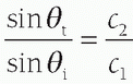
. For small angles, this can be approximated as image. Figure 14-4B illustrates the refraction angle when the speeds of sound in tissue 1 are greater than or less than tissue 2.

A situation called total reflection occurs when c2c1 and the angle of incidence of the sound beam with the boundary between two media exceeds an angle called the critical angle. In this case, the sound beam does not penetrate the second medium but travels along the boundary. The critical angle (θc) is calculated by setting θt = 90° in Snell’s law (equation above), producing the equation sin θc = c1/c2.


14.2.4 Scattering

Scattering arises from objects and interfaces within tissues that are about the size of the ultrasound wavelength or smaller. At low frequencies (1-5 MHz) wavelengths are relatively large, and tissue boundaries appear smooth or specular (mirror-like). A specular reflector represents a smooth boundary between two tissues. At higher frequencies (5-15 MHz), wavelengths are smaller, and on a smaller scale, the same boundaries manifest with irregular, non-normal interfaces causing echo reflection in many directions. This effect is enhanced with increased frequency. A non-specular reflector represents a boundary that presents many different angles to the ultrasound beam and of the returning echoes, only a fraction of the echo intensity will return to the transducer, resulting in a large signal attenuation (Fig. 14-5).

Many organs can be identified by a defined “signature” or “echo texture” caused by intrinsic structures that produce variations in the returning scatter intensity. Scatter amplitude differences from one tissue region to another result in corresponding brightness changes on the ultrasound display. In general, the echo signal amplitude from tissue or material depends on the number of scatterers per unit volume, the acoustic impedance differences at interfaces, the sizes of the scatterers, and the ultrasound frequency. Tissues generating higher scatter amplitude are called “hyperechoic” and tissues generating lower or no scatter amplitude tissues are called “hypoechoic” relative to the average background signal. Non-specular echo signals are more prevalent relative to specular echo signals when using higher ultrasound frequencies, making the images appear more echogenic and granular.


14.2.5 Absorption and Attenuation

Attenuation is the loss of intensity with distance traveled, caused by scattering and absorption of the incident beam. Scattering has a strong dependence with increasing ultrasound frequency. Absorption occurs by transferring energy to the tissues that result in heating or mechanical disruption of the tissue structure. The combined effects of scattering and absorption result in exponential attenuation of ultrasound intensity with distance traveled as a function of increasing frequency. When expressed in decibels (dB), a logarithmic measure of intensity, attenuation in dB/cm linearly increases with ultrasound frequency. An approximate rule of thumb for average ultrasound attenuation in soft tissue is 0.5 dB/cm times the frequency in MHz. Compared to a 1-MHz beam, a 2-MHz beam will have approximately twice the attenuation, a 5-MHz beam will have five times the attenuation, and a 10-MHz beam will have ten times the attenuation per unit distance traveled. Since the dB scale progresses
logarithmically to the base 10, the beam intensity is attenuated to the power of 10 with distance (See Fig. 14-6). Careful selection of the transducer frequency must be made in the context of the imaging depth needed for an exam. The loss of ultrasound intensity in decibels (dB) can be determined empirically for different tissues by measuring intensity as a function of distance traveled in centimeters (cm) and is the attenuation coefficient µ, expressed in dB/cm. For a given ultrasound frequency, tissues and fluids have widely varying attenuation coefficients chiefly resulting from structural and density differences, as indicated in Table 14-4 for a 1-MHz ultrasound beam.


FIGURE 14-5 Specular and non-specular boundary characteristics are partially dependent on the wavelength of the incident ultrasound. For long wavelengths, tissue boundary interactions are smooth and mirror-like. As the wavelength reduces with higher frequency ultrasound, the boundary becomes “rough” with non-perpendicular surfaces that result in diffuse scattering from the surface.


FIGURE 14-6 Ultrasound attenuation occurs exponentially with penetration depth and increases with increased frequency. The plots are estimates of a single frequency ultrasound wave with an attenuation coefficient of (0.5 dB/cm)/MHz of ultrasound intensity versus penetration depth. Note that the total distance traveled by the ultrasound pulse and echo is twice the penetration depth.

Another attenuation measure is the ultrasound HVT, the thickness of tissue necessary to attenuate the incident intensity by 50%. This is determined by taking the ratio of 3 dB (a factor of 2 or 50% on the dB scale) by the attenuation coefficient (dB/cm) for a specified frequency. As the frequency increases, the HVT decreases and the depth of penetration decreases, as illustrated by the examples below.


TABLE 14-4 ATTENUATION COEFFICIENT µ(dB/cm-MHz) FOR TISSUES ENCOUNTERED IN ULTRASOUND


TISSUE


µ (1 MHz)a


Air


1.64


Blood


0.2


Bone


7-10


Brain


0.6


Cardiac


0.52


Connective tissue


1.57


Fat


0.48


Liver


0.5


Muscle


1.09


Tendon


4.7


Soft tissue (average)


0.54


Water


0.0022


a For higher frequency operation, multiply the transducer frequency in MHz by the attenuation coefficient.


EXAMPLE 1: Calculate the approximate intensity HVT in soft tissue for ultrasound beams of 2 and 10 MHz.

Answer: Information needed is (1) the attenuation coefficient approximation 0.5 (dB/cm)/MHz and (2) the HVT intensity expressed as a 3 dB loss. Given this information, the HVT in soft tissue for an ultrasound beam of frequency f (MHz) is


EXAMPLE 2: Calculate the approximate intensity loss of a 5-MHz ultrasound wave traveling round-trip to a depth of 4 cm in the liver and reflected from an encapsulated air pocket (100% reflection at the boundary).

Answer: Using 0.5 dB/(cm-MHz) for a 5-MHz transducer, the attenuation coefficient is 2.5 dB/cm. The total distance traveled by the ultrasound pulse is 8 cm (4 cm to the depth of interest and 4 cm back to the transducer). Thus, the total attenuation is 2.5 dB/cm × 8 cm = 20 dB. The incident intensity relative to the returning intensity (100% reflection at the boundary) is


Therefore, IIncident = 100 IEcho.

The echo intensity is one-hundredth of the incident intensity in this example or -20 dB. If the boundary reflected 1% of the incident intensity (a typical value), the returning echo intensity would be (100/0.01) or 10,000 times less than the incident intensity, or -40 dB. Considering the depth and travel distance of the ultrasound energy, the detector system must have a dynamic range of 60 to 70 dB relative intensity (120 to 140 dB relative pressure) to reliably detect acoustic echoes generated in the medium. When penetration to deeper structures is important, lower frequency ultrasound transducers must be used.


14.3 ULTRASOUND TRANSDUCERS

Ultrasound is transmitted and received with a transducer array, comprised of hundreds of small ceramic elements with electromechanical (piezoelectric) properties, connected to controlling electronics, aligned in a row, and contained in a handheld hardened plastic housing.


14.3.1 Piezoelectric Materials

Piezoelectric materials are materials that can generate an internal electrical charge from applied mechanical stress. The term piezo is a Greek derivation for “press.” These same materials can exhibit the inverse piezoelectric effect with the internal generation
of mechanical strain in response to an applied electrical field. Ultrasound transducers for medical imaging applications employ a synthetic piezoelectric ceramic, lead-zirconate-titanate (PZT), or a silicon-based capacitive micromachined ultrasound transducer (CMUT).

PZT is a manufactured compound with an internal molecular dipole (positive and negative charge) asymmetrical crystal lattice structure. When expanded or compressed under a mechanical force, the small displacements create polarization in proportion to the stress that produced it. Re-orientation of the internal dipole structure generates a positive and negative charge on each of the surfaces of the PZT crystal (Fig. 14-7A). To detect ultrasound, electrode wires are attached to each surface to measure the surface charge variations resulting from the compression and rarefaction of returning ultrasound echoes, generating a potential difference on the order of 10s to 100s of µV (µV = one-millionth of a volt). To generate ultrasound, the same electrode wires on the PZT crystal use the inverse piezoelectric effect by applying a voltage with a polarity to cause contraction or expansion of the transducer crystal thickness as illustrated in Figure 14-7B.

An alternate, relatively new electromechanical method of producing ultrasound is with silicon-based CMUT materials. The basic element of a CMUT is a capacitor cell with a fixed electrode (backplate) and a free electrode (membrane) that uses electrostatic transduction. An alternating voltage applied between the membrane and the backplate creates a modulating electrostatic force that results in membrane vibration with the generation of ultrasound. In the receive mode, the membrane is subject to an incident ultrasound wave that results in a capacitance change detected as a voltage signal. The main advantages of CMUT compared to PZT are better acoustic matching with the propagation medium, which allows wider bandwidth capabilities, improved resolution, and potentially lower costs with easier fabrication. While only beginning to emerge in diagnostic medical ultrasound, CMUT transducers show great promise for improvements in efficiency, speed, multi-bandwidth operation, and volumetric imaging.


FIGURE 14-7 The piezoelectric element is comprised of aligned molecular dipoles. A. Under the influence of mechanical pressure from an adjacent medium (e.g., an ultrasound echo), the element thickness contracts (at the peak pressure amplitude), achieves equilibrium (with no pressure), or expands (at the peak rarefactional pressure) causing realignment of the electrical dipoles to produce positive and negative surface charge. Surface electrodes measure the amplitude of the charge in millivolt to microvolt output as a function of time in receive mode. B. An external voltage source (˜100 V) applied to the element surfaces over several microseconds causes compression or expansion from equilibrium by realignment of the dipoles in response to the electrical attraction or repulsion force in transmit mode.


FIGURE 14-8 A short-duration voltage spike causes the piezoelectric element to vibrate at its natural resonance frequency, f0, which is determined by the thickness of the transducer equal to ½λ. Low-frequency oscillation is produced with a thicker piezoelectric element.


14.3.2 Resonance Frequency, Damping, Absorbing and Matching Layers

Excitation of a PZT element is implemented with a voltage spike of 10-150 V over 1 to 2 µs with a polarity to re-orient dipoles and contract the crystal. Subsequent expansion and contraction result in vibration at a natural “resonance” frequency—dependent on crystal thickness. This is much like the way a “tuning” fork vibrates at a constant audible pitch (frequency) dependent on the distance between its tines. As shown in Figure 14-8, the PZT crystal thickness equal to one-half the wavelength of ultrasound is the preferred vibration frequency—thus, the manufactured thickness determines the center operating frequency. Crystal vibration will continue over an extended time at this natural frequency without any external contact, resulting in a long ultrasound pulse. In practice, many transducer elements are aligned in an array and individually controlled as shown in Figure 14-9. Each transducer element
functions in an excitation mode to transmit ultrasound energy, and in a reception mode to receive ultrasound energy. To be able to use the pulse-echo format, there is a need to shorten the pulse.


FIGURE 14-9 A. A singleelement crystal with surface electrodes, showing the thickness, width, and height dimensions. B. A section of a multielement transducer array at equilibrium (blue), thickness mode contraction (green), and expansion (red). With thickness mode variation there is also variation in the width and height of the array. The dashed double arrows represent the equilibrium dimensions.

Other layers are necessary to control the spatial and transmission characteristics of the ultrasound pulse (Fig. 14-10). Layered on the backside of each element is a damping block to attenuate the transducer vibration duration in order to produce an ultrasound pulse with a short spatial pulse length (SPL). This preserves detail of organ boundaries and echogenic anatomy carried by the returning echoes. Dampening of the transducer crystal vibration (also known as “ring-down”) introduces a range of frequencies above and below the center frequency and results in a broadband frequency spectrum. A term called the “ Q-Factor” describes the ratio of the center frequency and the bandwidth of the pulse, as: image
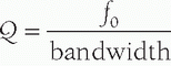
, where f0 is the center frequency and the bandwidth is the width of the frequency distribution. A high “Q” transducer operation has a narrow bandwidth and a long spatial pulse width, which is good for evaluating frequency shifts such as are used in pulsed Doppler studies for measuring blood velocities (Section 14.8). A low “Q” transducer has heavy damping and a rapid ring-down of the crystal vibration to achieve a short SPL for imaging studies.

Behind the damping block is an absorbing layer, which is present to reduce the backside-produced ultrasound energy and to attenuate stray ultrasound signals reflected from the transducer housing. On the front side of the transducer array is the matching layer, which provides the interface between the PZT element and the tissue. It consists of one or more layers of materials with acoustic properties intermediate to that of soft tissue and transducer element composition to minimize acoustic impedance differences and maximize the transmission of ultrasound into the tissues. The thickness of each layer is equal to ¼ wavelength, determined from the center operating frequency of the transducer and speed characteristics of the matching layer. For example, the wavelength of sound in a matching layer material with a speed of sound of 2,000 m/s for a 5-MHz ultrasound beam is 0.4 mm. The optimal matching layer thickness is equal to ¼λ = ¼ × 0.4 mm = 0.1 mm. In addition to the matching layer, acoustic coupling gel (with acoustic impedance similar to soft tissue) is used between the transducer and the skin of the patient to eliminate air pockets that could attenuate and reflect the ultrasound beam.


FIGURE 14-10 A. The transducer is comprised of a housing, electrical insulation, and a composite of active element layers, including the PZT crystal, damping block and absorbing material on the backside, and a matching layer on the front side of the multielement array. B. The ultrasound spatial pulse length is based upon the damping material causing a ring-down of the element vibration. For imaging, a pulse of 2 to 3 cycles is typical, with a wide frequency bandwidth, while for Doppler transducer elements, less damping provides a narrow frequency bandwidth.


14.3.3 Broad Bandwidth “Multifrequency” Transducer Operation

Unlike the simple resonance transducer design of pure PZT, the multifrequency piezoelectric crystal element is manufactured with many small rods and backfilled with an epoxy resin to create a smooth surface. The acoustic properties of these composite elements are closer to tissue than a pure PZT material and thus provide a greater transmission efficiency of the ultrasound beam without resorting to multiple matching layers. In terms of excitation, by varying the transmit voltage to the crystal electrodes in a specific way, the transducer crystal can be made to expand and contract over a selectable range of frequencies. Coupled with digital signal processing, “multifrequency” or “multihertz” transducer operation over a known frequency range is enabled, whereby the center frequency can be selected in the transmit mode. Broadband multifrequency transducers have bandwidths that exceed 80% of the center frequency (Fig. 14-11). For a given transducer, multifrequency operation allows the sonographer to interactively choose the appropriate frequency to emphasize spatial resolution or depth of penetration based upon the needs of the examination. Multihertz transducers are often identified with the frequency range of operation, for example, C4-10, where the letter indicates the transducer array type (e.g., C = convex) and the numbers identify the operational frequency range.

Excitation of the multifrequency transducer elements is accomplished with a short square wave burst of approximately 150 V with one to three cycles, unlike the voltage spike used for resonance transducers. This allows the transmit frequency to be selected within the limits of the transducer bandwidth. Likewise, the broad bandwidth response permits the reception of echoes within a selected range of frequencies. For instance, ultrasound pulses can be transmitted at a low frequency and the echoes received at higher frequency as is accomplished with harmonic imaging (see Section 14.6).


14.3.4 Transducer Arrays

Most medical ultrasound systems employ transducers with linear, curvilinear (convex), or phased arrays, comprised of 10’s to 1,000’s of individual crystals. Transducer arrays operate over many selectable frequencies with multihertz broadband operation, have various physical dimensions and “footprints,” and provide different image display formats.


FIGURE 14-11 Multifrequency transducer transmit and receive response to operational frequency bandwidths allows the operator to select an appropriate transmit and receive frequency depending on the type of exam, type of transducer, the transducer bandwidth range, and the need for penetration depth (selecting lower frequency) or spatial resolution (selecting higher frequency). The transducer response shown has a selectable frequency range of 4 to 10 MHz.


FIGURE 14-12 A. The linear array transducer activates a subgroup of transducer elements to produce an ultrasound beam directed perpendicular to the array, repeating with incremental shifting of the subgroup element by element. A rectangular field of view is produced. B. A common linear array transducer with a 6 to 15 MHz range of operation is pictured.

Linear array transducers activate a subset of elements in a group, producing a single transmit beam at one location perpendicular to the aperture, and then listen for echoes in the receive mode. Within a fraction of a second when all echoes are received from the greatest depths, the next pulse is created by activating another element aperture group that is incrementally shifted along the transducer array, and the process repeats on the order of thousands of times per second to generate a rectangular image format with real-time frame rates and data acquisition (Fig. 14-12A). Linear arrays are comprised of hundreds to thousands of transducer elements, have small to large form factors, and generally operate at higher frequencies, from 5 to 20 MHz. These transducers are suited for imaging superficial structures such as the eyes, joints, muscles, and proximal blood vessels and for performing ultrasound-guided biopsy procedures. A 6-15 MHz linear array transducer is shown in Figure 14-12B. A small footprint “hockey stick” linear array is shown in Figure 14-31.

Curvilinear array transducers (often called convex arrays) have hundreds of elements in a convex geometry with a relatively larger housing and footprint than linear arrays. Like the linear array, a subset of piezoelectric elements defining an aperture are sequentially activated, producing a trapezoidal image format with an increased field of view at both proximal and distal depths as shown in Figure 14-13A. These transducers are ideal for imaging intraabdominal organs such as the liver, spleen, kidneys, and bladder that need large FOV coverage. Low to mid-range frequencies (1-10 MHz) are used. For depth penetration with larger patients, low-frequency operation limits spatial resolution, and at greater depths the ultrasound beam sampling becomes sparse. A 1-6 MHz curvilinear array is pictured in Figure 14-13B.

Phased array transducers (also known as sector scanners) are typically comprised of a tightly grouped array of ˜60 to hundreds of transducer elements in a 3- to 5-cm-wide enclosure. All transducer elements are involved in producing the ultrasound beam and recording the returning echoes. The ultrasound beam is electronically steered by adjusting the delays applied to the individual transducer elements as illustrated in Figure 14-14A. This time delay sequence is varied from one transmit pulse to the next in order to incrementally change the sweep angle across the FOV in a sector scan format, as shown in Figure 14-14B. In receive mode, returning echoes are detected by all transducer elements in the array. Phased array transducers mostly operate at lower frequencies over a range of 1-5 MHz (although some operate at higher frequencies from 8 to 12 MHz). A narrow to wide sector field of view
can be interactively selected by the operator. The smaller physical dimension of the transducer array is useful for access to intercostal acoustic windows when performing heart and thoracic imaging exams. With a sector-scan format, the FOV dimension can be limited in regions proximal to the transducer array. A 1-5 MHz phased array transducer is shown in Figure 14-14C.


FIGURE 14-13 A. The curvilinear (also known as convex) array operates with subgroup transducer element excitation, like the linear array. A convex arrangement produces a trapezoidal field of view, with good coverage proximally and extended coverage distally. B. A common curvilinear array transducer with a 1 to 6 MHz range of operation is pictured.
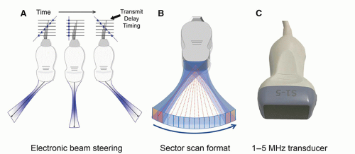


FIGURE 14-14 A. A phased array transducer produces a beam from the near simultaneous excitation of all array elements. The beam can be electronically steered across the FOV using transmit delay excitation patterns—three are shown. B. A sector scan format is produced with incremental time delay patterns to control the direction and number of lines across the FOV. C. A common phased array transducer with a 1-5 MHz range of operation is pictured.

Other transducer arrays often found in a radiology ultrasound imaging suite include intracavitary array probes (Fig. 14-15A) for internal imaging, and mechanically scanned curved arrays in a larger protective housing (Fig. 14-15B) for volumetric imaging. Intracavitary probes are designed to operate inside a body cavity, have specialized shapes, and operate with a linear or phased array sequence based upon transducer array configurations. The proximity of the transducer to the tissue region allows a higher frequency range (5-8 MHz), with a wide field of view, and excellent image resolution. These transducers are used in trans-vaginal, trans-rectal, and
intraoral applications. The mechanically scanned curved array transducer is commonly used in obstetrical evaluations for 3D volume image acquisitions. Mechanical scanning of the curved array occurs simultaneously with 2D image acquisition and is synchronized to provide volumetric sampling over a ˜90° by ˜90° FOV range as a function of time. Shaded surface and volumetric rendering generate real-time 3D movies of the fetus, as discussed in Section 14.6.

There are many other transducer probes and types not discussed here, such as annular arrays, fully 2D electronic matrix arrays with thousands of transducer elements for real-time 3D and 4D imaging of the heart, and other specialized applications (Szabo and Lewin, 2013).


FIGURE 14-15 Intracavitary array probes exist in a variety of shapes and acquisition geometries to directly image internal organs with cavity access. A. Endovaginal curvilinear array with very wide 150° FOV and 5-9 MHz range of operation. B. Endovaginal probe using mechanically scanned curved array transducer for 3D imaging acquisitions, with 5-9 MHz range. C. Mechanically scanned curved array transducer assembly for the acquisition of 3D volumetric imaging of the fetus, with a 4-8 MHz operational range.


14.4 ULTRASOUND BEAM PROPERTIES

The ultrasound beam propagates as a longitudinal wave from the transducer surface into the propagation medium and exhibits two distinct beam patterns: a slightly converging beam out to a distance determined by the geometry and frequency of the transducer (the near field), and a diverging beam beyond that point (the far-field), as shown in Figure 14-16.


14.4.1 The Near Field

The near field, also known as the Fresnel zone, is adjacent to the transducer face and has a converging beam profile. Beam convergence occurs because of multiple constructive and destructive interference patterns of the ultrasound waves from the transducer surface. “Huygens’ principle” describes a large transducer surface as an infinite number of point sources of sound energy where each point is characterized as a radial emitter (see Fig. 14-16, left middle diagram). As individual wave patterns interact, the peaks and troughs from adjacent sources constructively and destructively interfere causing the beam profile to be collimated. The ultrasound beam path is thus
largely confined to the dimensions of the active portion of the transducer surface, with the beam converging to approximately half the transducer area at the end of the near field. The near field length is dependent on the transducer area and inversely proportional to propagation wavelength, so higher transducer frequency results in an extended near field. Lateral resolution (the ability of the system to resolve objects in a direction perpendicular to the beam direction) depends on the lateral beam dimension and is best at the end of the near field for an unfocused transducer element aperture (e.g., a subgroup of linear array transducer elements fired simultaneously).

Pressure amplitude changes caused by ultrasound propagation in the near field are very complex, produced by the individual transducer element excitations and the constructive and destructive interference wave pattern interactions of the ultrasound beam. Pressures vary rapidly from peak compression to peak rarefaction several times during transit through the near field. Peak ultrasound pressure occurs at the end of the near field, corresponding to the minimum beam area.


FIGURE 14-16 A linear array transducer subgroup excitation (top) and the expanded beam profile (middle) shows the near-field and far-field characteristics of the ultrasound beam. The near field is characterized as a collimated beam, and the far field begins when the beam diverges. Point emitters (left middle) generate constructive and destructive interference patterns that cause beam collimation and large pressure amplitude variations in the near field (lower diagram). Beam divergence occurs in the far field, where pressure amplitude monotonically decreases with propagation distance.


14.4.2 The Far Field

The far-field, also known as the Fraunhofer zone, begins at the distance from the transducer where the beam diverges, and lateral resolution degrades. The angle of divergence is directly proportional to the wavelength and inversely proportional to the transducer area. Less beam divergence occurs with higher-frequency and larger sub-element excitations in a linear array. Ultrasound intensity in the far-field decreases monotonically with distance (Fig. 14-16 bottom illustration).


14.4.3 Transducer Array Beam Focusing

Transducer elements in a linear array that are fired simultaneously produce an effective transducer width equal to the sum of the widths of the individual elements. Individual beams interact via “constructive” and “destructive” interference to produce a
collimated beam that has properties like the properties of a single crystal area transducer of the same size. Thus, for a subgroup of simultaneously fired transducers in a linear array, the focal distance is a function of the transducer area (height/width) and the transducer frequency. With slight differences in excitation time for individual elements in the subgroup aperture (or full phased array), wave interactions and summations can focus the beam.


Transmit Focus

Array transducer electronics can apply specific timing delays between transducer elements in a subgroup for linear and curvilinear array transducers, and for all elements in a phased array transducer to cause the beam to converge at a specified closer distance. A shallow focal zone (close to the transducer surface) is produced by firing outer transducer elements before the inner elements in a symmetrical pattern, as shown in Figure 14-17A for a phased-array transducer (note that these principles also apply for the subgroup aperture elements in a linear or curvilinear array). Focal distances at greater depth are achieved by reducing the delay time differences amongst the transducer elements, resulting in more distal beam convergence.


FIGURE 14-17 Transmit and Receive focusing. A. Transmit focusing is achieved by implementing a programmable delay time (beamformer electronics) for the excitation of the individual transducer elements in a concave pattern with outer elements energized first. The individual ultrasound pulses converge to a minimum beam diameter (the focal distance) at a predictable depth in tissue. B. Dynamic receive focusing uses receive beamformer electronics to dynamically adjust delay times for processing the received echo signals. This compensates for differences in arrival time across the array as a function of time (depth of the echo) and results in phase alignment of the echo signals by all elements to achieve a good signal output as a function of time.


Receive Focus

The echoes received by the active transducer elements are summed together to create the ultrasound signal from a given depth as a function of time. Echoes received at the edge of the array travel a slightly longer distance than those received at the center, particularly at shallow depths, and are received later, causing phase misalignment during the summation of the individual transducer responses. Dynamic receive focusing is a method to align the phase by introducing electronic delays continuously as a function of depth (time). At shallow depths, delays between adjacent transducer element reception times are largest. With greater depth the returning beam is less concave, so the delays are less, as shown in Figure 14-17B. This is for both linear (subgroup) and phased array transducer operation.


Dynamic Aperture

The lateral spatial resolution of the linear array beam varies with depth, dependent on the linear dimension of the transducer width (aperture). A process termed dynamic aperture increases the number of active receiving elements in the linear array with reflector depth so that the lateral resolution does not degrade with the depth of propagation.


14.4.4 Side Lobes and Grating Lobes

Side lobes are unwanted emissions of ultrasound energy directed away from the main pulse, caused by the expansion and contraction of the transducer elements in the width and height dimensions during thickness contraction and expansion as explained earlier (see Fig. 14-9B). Side lobe emissions occur in a forward direction along the main beam (Fig. 14-18A). Individual transducer element widths that are less than ½ wavelength reduce the intensity of side lobe emissions. Side lobe emission intensity is also reduced with lower Q transducer operation (high damping) and when the amplitude of peripheral transducer element excitation voltages are less relative to the central element excitation voltages.


FIGURE 14-18 Side lobes and grating lobes. A. Side lobes represent ultrasound energy produced outside of the main ultrasound beam along the same beam direction caused by height and width variations of the transducer elements. B. Grating lobes represent emission of energy at large angles relative to the direction of the beam caused by the discrete nature of the multielement transducer array. At the edges of the array, energy is emitted that does not undergo interference as shown by the inset diagram. The grating lobe intensity is low relative to the intensity of the main beam or side lobes.
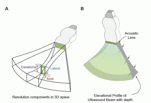

Grating lobes result when ultrasound energy is emitted far off-axis by multielement arrays and are a consequence of the non-continuous, discrete element transducer surface. The grating lobe effect is equivalent to placing a grating in front of a continuous transducer element, producing coherent waves directed at a large angle away from the main beam (Fig. 14-18B). This misdirected energy of relatively low amplitude can reflect from off-axis tissue boundaries with high impedance mismatch and return to the transducer array.

In the receive mode of transducer operation, echoes generated from the side and grating lobes are unavoidably remapped as coming from the main beam, which can introduce artifacts in the image (see Section 14.9). For transducer operation with a narrow frequency bandwidth (high Q) the side lobe energy is a significant fraction of the total beam. In pulsed mode operation, the low Q, broadband ultrasound beam produces a spectrum of wavelengths that reduces the emission of side lobe energy.


14.4.5 Spatial Resolution

In ultrasound, the major factor that limits the spatial resolution and visibility of detail is the volume of the acoustic pulse. The axial, lateral, and elevational (slice-thickness) dimensions determine the minimal volume element (Fig. 14-19). Each dimension has an effect on the resolvability of objects in the image.


Axial Resolution

Axial resolution (also known as linear, range, longitudinal, or depth resolution) refers to the ability to discern two closely spaced objects in the direction of the beam. Achieving good axial resolution requires that the returning echoes from adjacent boundary reflectors be distinct without overlap. The ultrasound SPL, a product of the wavelength and the number of cycles emitted per pulse, determines axial resolution.


FIGURE 14-19 A. The axial, lateral, and elevational (slice-thickness) contributions in three dimensions are shown for a phased-array transducer ultrasound beam. Axial resolution, along the direction of the beam, is independent of depth; lateral resolution and elevational resolution are strongly depth dependent. Lateral resolution is determined by transmit and receive focus electronics; elevational resolution is determined by the height of the transducer elements. At the focal distance, axial is better than lateral, and lateral is better than elevational resolution. B. Elevational resolution profile with an acoustic lens across the transducer array produces a weak focal zone in the slice-thickness direction.


FIGURE 14-20 Axial resolution is equal to ½ SPL. Tissue boundaries that are separated by a distance greater than ½ SPL produce echoes from the first boundary that are completely distinct from echoes reflected from the second boundary, whereas boundaries with less than ½ SPL result in overlap of the returning echoes. Higher frequencies reduce the SPL and thus improve the axial resolution, as shown in the lower diagram.

Shorter pulses can be achieved with greater damping of the transducer element (to reduce the pulse duration and number of cycles) or with higher frequency (to reduce wavelength). The minimal required separation distance between two reflectors is one-half of the SPL to avoid the overlap of returning echoes, as the distance traveled between two reflectors is twice the separation distance. Objects spaced closer than ½ SPL will not be resolved (Fig. 14-20).

For imaging applications, the ultrasound pulse typically consists of three cycles. In tissue at 5 MHz (wavelength of 0.31 mm), the SPL is about 3 × 0.31 = 0.93 mm, which provides an axial resolution of ½ (0.93 mm) = 0.47 mm. At a given frequency, shorter pulse lengths require heavy damping and low Q, broad bandwidth operation. For a constant damping factor, higher frequencies (shorter wavelengths) give better axial resolution, but the imaging depth is reduced due to higher attenuation. The axial resolution remains constant with depth.


Lateral Resolution

Lateral resolution, also known as azimuthal resolution, refers to the ability to discern two closely spaced objects perpendicular to the beam direction as distinct. The beam width determines the lateral resolution (see Fig. 14-21). Since the beam width varies with distance from the transducer in the near and far-field, the lateral resolution is depth-dependent. The best lateral resolution occurs at the near field-far field interface. At this depth, the effective beam width is approximately equal to ½ the effective transducer width. In the far-field, the beam diverges and substantially reduces the lateral resolution.


FIGURE 14-21 Lateral resolution is a measure of the ability to discern objects perpendicular to the direction of beam travel and is determined by the beam diameter. Point targets in the beam are averaged over the effective beam diameter in the ultrasound image as a function of depth. Best lateral resolution occurs at the focal distance; good resolution occurs over the focal zone.

As the beam width can be selectively varied as a function of depth with adjustable delay times for exciting the transducer elements (see Fig. 14-17A), lateral resolution can be improved. Moreover, multiple transmit/receive focal zones can be implemented to maintain lateral resolution as a function of depth for both linear and phased array transducer operation (Fig. 14-22). Each focal zone requires a separate pulse-echo sequence to acquire data. This is accomplished by acquiring data along one beam direction multiple times equal to the number of transmit focal zones, accepting only the echoes within each focal zone, and merging the data. Increasing the number of focal zones improves overall in-focus lateral resolution with depth, but the amount of time required to produce an image increases, with a consequent reduction in frame rate and/or number of scan lines per image.


Elevational Resolution

The elevational or slice-thickness dimension of the ultrasound beam is perpendicular to the image plane. Slice thickness plays a significant part in image resolution, particularly with respect to volume averaging of acoustic details in the regions close to the transducer and in the far-field beyond the focal zone. Elevational resolution is dependent on the transducer element height in much the same way that the lateral resolution is dependent on the transducer element width as shown in Figure 14-19B. The slice thickness dimension has the poorest
resolvability for array transducers. The use of an acoustic lens across the entire array can provide improved elevational resolution at a fixed focal distance. Unfortunately, this compromises resolution before and after the elevational focal zone due to partial volume averaging.


FIGURE 14-22 Linear and phased-array transducers have multiple user-selectable transmit and receive focal zones implemented by the beamformer electronics. In this example, a phased array transducer is illustrated. Each focal zone requires the transmit beamformer excitation of the active array for a given focal distance. Subsequent processing meshes the independently acquired data to enhance the lateral focal zone over a greater distance. Good lateral resolution over an extended depth can be achieved at the expense of reduced image frame rate.

Multiple linear array transducers with five to seven rows, known as 1.5D transducer arrays, have the ability to steer and focus the beam in the elevational dimension. Elevational focusing is implemented with phased excitation of the outer to inner arrays to minimize the slice-thickness dimension at a given depth (Fig. 14-23). By using subsequent excitations with different focusing distances, multiple transmit
focusing can produce smaller slice thickness over a range of tissue depths. A disadvantage of elevational focusing is a frame rate reduction penalty required for multiple excitations to build one image. The increased width of the transducer array also limits positioning flexibility. Extension to full 2D transducer arrays with enhancements in computational power allows 3D imaging with more uniform resolution throughout the image volume.


FIGURE 14-23 Elevational resolution with multiple transmit focusing zones is achieved with “1.5D” transducer arrays to reduce the slice-thickness profile over an extended depth. Five to seven rows of discrete arrays replace the single array. Phase delay timing provides focusing in the elevational plane, like that used for lateral transmit and receive focusing.

Only gold members can continue reading. Log In or Register to continue

Stay updated, free articles. Join our Telegram channel

May 16, 2021 | Posted by in GENERAL RADIOLOGY | Comments Off on Ultrasound

Full access? Get Clinical Tree

Get Clinical Tree app for offline access