Visualizing White Matter Pathways in the Living Human Brain: Diffusion Tensor Imaging and Beyond

Biologic connectionism holds as its central tenet that the cognitive, behavioral, and motor functions of the brain are derived from the complex interconnections of simple neural processing units. Much can be learned about the human mind through the study of the brain’s connections in normal and diseased states. This article summarizes the essential features of the tensor model of diffusion, outlines newer approaches to overcoming the limitations of the tensor, and provides normal and clinical examples of white matter anatomy derived using diffusion tensor imaging and more sophisticated high angular resolution diffusion imaging methods. Diffusion MR imaging is a powerful adjunct to techniques for studying brain function.

Through its superb tissue contrast, magnetic resonance imaging (MR imaging) has revolutionized the scientific and clinical study of the human brain. By exploiting differences in proton density, T ₁ and T ₂ relaxation, and macroscopic flow, abnormalities can be localized to a resolution that is typically on the order of 1 mm. Much of the brain’s function, however, derives from its organization at much smaller spatial scales. The normal cerebral cortex and deep gray matter contain more than 100 billion neuronal cell bodies and their supporting structures. The information-carrying portion of the white matter consists of axons, which form an elaborate network of circuits interconnecting processing units within gray matter and relaying information to the body by way of the spinal cord and cranial nerves. Because neurologic and psychiatric disorders affect white matter in different ways, the ability to visualize the complex “wiring” of the brain provides an important window into the operation of the human mind.

Diffusion MR imaging differs from other MR imaging modalities in that it can be used to infer information about structures much smaller than the spatial resolution of the image. It may therefore be considered a “microstructural” imaging technique. Conventional techniques for eliciting the connectivity between different brain regions are based on histologic tissue analysis or on meticulous dissection of post-mortem specimens. Such approaches are not only invasive and not applicable to the in vivo study of the human brain but are also highly labor intensive and subject to the inherent problems associated with tissue fixation. In contrast, diffusion MR imaging is a tool for straightforward, rapid “virtual dissection” of the living human brain.

The purpose of this article is fourfold: (1) to provide a brief overview of the theoretic principles underlying diffusion tensor imaging (DTI) and newer non-tensor diffusion MR imaging methods, such as high angular resolution diffusion imaging (HARDI); (2) to review the white matter tracts that are commonly visualized in the normal human brain using DTI and HARDI; (3) to use callosal agenesis as a clinical example of how diffusion MR imaging can be used in the study of aberrant white matter connectivity, and finally; (4) to summarize several current research directions in diffusion MR imaging that may ultimately find practical use in systems neuroscience and in clinical neuroradiology.

Magnetic resonance diffusion imaging techniques

Diffusion weighting

Water molecules, the principal constituents of the brain, are in constant motion caused by random thermal fluctuation. Within an artificial environment such as a test tube filled with pure water, molecular mobility can be quantified by MR imaging using the diffusion (or self-diffusion) coefficient, a physical constant that expresses the mean displacement of water molecules in a given time interval. In biologic tissues, the motion of water is influenced not only by properties inherent to the molecules themselves, but also by the surrounding environment in which diffusion takes place. In this setting, diffusion can be described using the apparent diffusion coefficient (ADC), distinguished from the self-diffusion coefficient in that it includes the empiric aggregate of all factors that determine the nature of local molecular diffusion. ADC is a tissue-specific biologic marker whose value varies throughout the brain, depending on active transport and passive diffusion of water, microscopic barriers to diffusion such as cell membranes and organelles, and compartmentalization of water within cell bodies, axons, and glia . Expressed in units of area per unit time (typically mm ²/s), the ADC can be viewed as a measurement of the average rate of diffusion within a voxel.

In a homogeneous medium in which protons are equally likely to diffuse in any direction, diffusion is said to be isotropic, and a single measurement of ADC suffices to characterize the medium. In contradistinction, diffusion in white matter tracts is directionally dependent— that is, the trajectory of molecules caused by thermal motion is more likely to occur along certain orientations than others. These three-dimensional constraints on the movement of water protons cause diffusion to exhibit directional anisotropy . The anisotropy of diffusion can be measured using MR imaging and has an important biologic meaning—the average direction of proton diffusion preferentially aligns with the orientation of axonal fibers within white matter tracts. To adequately characterize the directional anisotropy, it is necessary to obtain measurements of ADC along several different directions. Heuristically, it is thus useful to view ADC as a surface in three dimensions that varies depending on the angular direction in which it is measured. The information encoded by the shape of the ADC surface allows inference of the orientational structure of the underlying neural architecture.

The critical element of an MR pulse sequence that sensitizes it to proton diffusion is the diffusion gradient. Diffusion gradients can be incorporated into virtually any pulse sequence, but are most commonly used in a spin-echo experiment by placing identical gradient pulses before and after the 180° refocusing pulse. It is important to point out that diffusion gradients are applied independently and in addition to the phase-encoding and readout gradients used for spatial encoding and typically have much larger magnitudes. Mathematically, the diffusion gradient is a vector quantity that has magnitude (the strength of the diffusion gradient) and direction (the angular orientation in which the gradient is applied). Applied along any single orientation, the diffusion gradient causes the signal to be attenuated according to the equation

S/S0=e−b ADC,
S / S 0 = e − b ADC ,

where S is the measured diffusion-weighted signal, S ₀is the signal that would be obtained without diffusion weighting, and b is the strength of the diffusion-weighting for the experiment (determined by the timing and strength of the diffusion gradients). Larger values of ADC result in greater signal attenuation. This equation allows the recovery of the ADC value for any directional diffusion measurement.

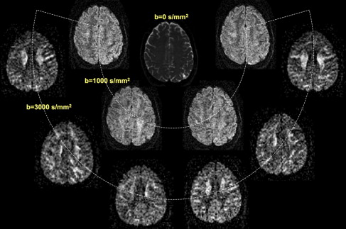
Overall the magnitude of the diffusion-weighted signal depends on two factors: (1) the three-dimensional angular orientation in which the diffusion gradients are applied during image acquisition, and (2) the strength of diffusion weighting applied, as parameterized by the b value for the acquisition. The strength, duration, and relative timing of the diffusion gradients with respect to the 180° refocusing pulse determine the b value. Fig. 1 illustrates the effect of these two parameters on the appearance of a diffusion-weighted image in a normal adult volunteer. For any specific b value, the resulting image contrast depends on the relative angular difference between individual fiber tracts and the direction of diffusion weighting. For a fixed direction of the diffusion gradient, increasing the value of b results in progressive signal attenuation from molecules diffusing over smaller and smaller distances. In general, larger b values impart higher overall contrast and greater sensitivity to directional encoding to diffusion-weighted images.

In what follows, the authors refer to the process of systematically varying the strength and direction of the applied diffusion gradients as one of obtaining diffusion-encoded images. Each diffusion encoding yields a single diffusion-weighted image whose intensity is a function of fiber orientation and the length scale over which diffusion is probed. To characterize the three-dimensional structure of diffusion, it is necessary to acquire multiple diffusion-encoded images along different orientations, and to make certain assumptions about the properties of diffusion in the brain. Depending on the assumed nature of diffusion, it is possible to synthesize a set of measured diffusion-weighted images in different ways so as to ultimately characterize the underlying white matter architecture.

Diffusion tensor imaging

To date the diffusion tensor remains the most widely applied mathematic model used to represent the angular variability of diffusion in three dimensions . Equivalent to assuming a Gaussian probability for diffusion along any single direction, the tensor effectively fits the angular variation of the ADC to the geometric shape of a three-dimensional ellipsoid. The six unique parameters that define the tensor are deduced from at least six diffusion-encoded images acquired along non-collinear directions .

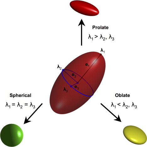
An intuitive and biologically meaningful parameterization of the diffusion ellipsoid results when the tensor is subjected to a mathematic operation termed eigendecomposition . As illustrated in Fig. 2 , this description of the tensor recasts the ellipsoid in terms of a unique set of three eigenvectors that represent the orientations of the major, medium, and minor principal ellipsoid axes, and three corresponding eigenvalues that quantify the value of the ADC along each axis. Depending on the magnitude of the eigenvalues, the diffusion ellipsoid may take on one of three basic shapes . When diffusion is equally likely along any direction, the ellipsoid is nearly spherical. Alternatively, when there is a single dominant direction for diffusion, as may be the case for a large and coherently oriented fiber tract, the ellipsoid is cigar-shaped (prolate). Finally, if diffusion is hindered along one axis but equally likely along the other two, the ellipsoid assumes a pill-shaped morphology (oblate). In fact, any tensor can be decomposed as a sum of these three cardinal shapes.

The two most widely used numeric descriptors of the tensor, fractional anisotropy (FA) and major axis, are also easily interpreted using the geometric parameterization of the diffusion ellipsoid. FA is calculated from the three eigenvalues and characterizes the degree to which the diffusion ellipsoid is anisotropic. When the large majority of fibers within any single voxel are organized along a single direction, the ellipsoid is long and narrow. The FA in this case is large, approaching its maximum value of 1. At the opposite extreme, when diffusion is nearly isotropic and the tensor is roughly spherical in morphology, the value of FA approximates zero. The other important parameter derived from the tensor is the major axis of the diffusion ellipsoid. This is given by the angular orientation of the eigenvector that corresponds to the largest eigenvalue (the principal eigenvector), and defines the direction in which the diffusion of water is least hindered. It is worth noting that FA is a putative marker of fiber density and myelination , and the principal eigenvector reflects the dominant orientation of white matter fascicles within each voxel.

To facilitate visual interpretation of diffusion tensor data, diffusion ellipsoid parameters are often used to derive color-encoded directional anisotropy maps. To construct these images, the principal axis of the diffusion ellipsoid for each voxel is converted to a unique color in RGB (red-green-blue) colorspace. The intensity of the assigned color is then weighted according to the value of FA. In the most commonly applied color scheme , used for the construction of the anisotropy maps shown in Figs. 3 and 4 , the anterior–posterior orientation is assigned to green, the left–right orientation is assigned to red, and the craniocaudal orientation is assigned to blue. As these images illustrate, highly isotropic diffusion within the cerebrospinal fluid spaces is characterized by small values of FA, and thus appears black in the color FA maps. The brightest voxels, in contrast, correspond to tightly packed, highly oriented, and largely myelinated white matter bundles, such as the corpus callosum. Because cortical and deep gray matter structures contain primarily cell bodies with no well-defined orientation, these areas have low anisotropy and are seen as dark pixels with no single dominant direction of diffusion on color FA maps.

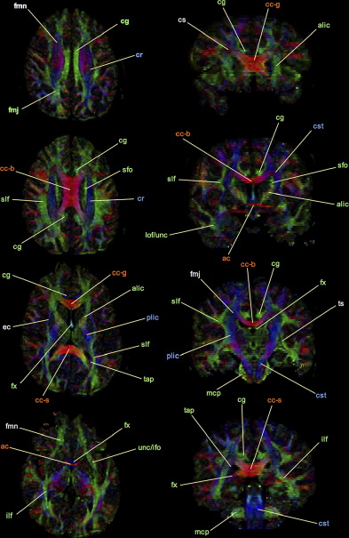
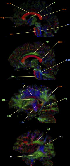
Careful inspection of Figs. 3 and 4 also demonstrates a substantial drawback of the tensor model. In areas in which fiber tracts cross, diverge, bend, or are otherwise partial volume-averaged within a single voxel, there is a relative falloff in anisotropy in comparison to surrounding white matter. This “artifactual” reduction of FA in regions of complex white matter architecture precludes accurate numeric quantitation of single-tract anisotropy and presents a significant obstacle to fiber tracking algorithms (see later discussion) . For example, this has been shown to interfere with DTI fiber tracking of many portions of the corticospinal tract in clinical applications, such as presurgical white matter mapping of patients who have brain tumors . Decreasing voxel size may help to reduce partial volume averaging of fiber tracts in some brain regions, but requires sacrificing signal-to-noise ratio (SNR) and yields less accurate tensor estimates. Moreover, axonal projections in certain brain regions, such as the centrum semiovale and the highly compact brainstem decussations, are known to interdigitate at a spatial scale that is orders of magnitude smaller than can be resolved using MR imaging.

High angular resolution diffusion imaging

One seemingly straightforward approach to recovering the subvoxel white matter architecture lost in the tensor model is to fit more than one tensor to directional measurements of the ADC. Unfortunately multitensor fitting is numerically challenging, and more important, the peaks of the ADC function may not actually correspond to dominant directions of distinct fiber populations . The shortcomings of multitensor models have recently spawned the development of several novel methods for recovering multiple fiber orientations using measurements of diffusion obtained at a fixed b value. Collectively referred to as techniques for high angular resolution diffusion imaging (HARDI), these have shown great promise and are currently the subject of intense research. The most popular methods that have been developed include q-ball imaging (QBI) , spherical deconvolution , FORECAST , persistent angular structure , and the diffusion orientation transform . These approaches each rely on a different assumption about the underlying probability of water diffusion, but together share the common goal of overcoming the inability of the tensor to represent more than one fiber orientation.

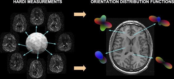
Data acquisition for HARDI is similar to DTI in that measurements are obtained at a fixed value of diffusion weighting b. Unlike DTI, however, HARDI uses much larger b-values (b = 3000 mm ²/s or higher) and requires that dozens or even hundreds of diffusion-weighted measurements be obtained to separately resolve subvoxel fiber populations. As illustrated schematically in Fig. 5 , diffusion encodings are acquired at points uniformly distributed over the surface of a sphere and synthesized to reconstruct a three-dimensional surface termed the orientation distribution function (ODF). This surface is analogous to the diffusion ellipsoid in that it quantifies the likelihood of diffusion along any angular direction, and its peaks coincide with the orientations of distinct fiber populations.

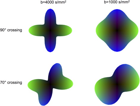
Akin to spatial resolution, a related but separate concept important for the interpretation of HARDI ODFs is that of angular resolution . Ideally, two crossing subvoxel fiber populations would result in an ODF that is comprised of two intersecting lines. In practice, however, the contribution of each population to the ODF has a finite width because of the true underlying coherence of diffusion (ie, “anisotropy”) and the measurement uncertainty in the directional estimates. As discussed, the magnitude of diffusion weighting determines the spatial scale over which water diffusion is evaluated. The most significant contribution of diffusion-weighted image contrast when b values of 3000 mm ²/s or higher are used is from the fraction of water molecules that, on average, are coincident with the direction of encoding over a long distance. As the value of b decreases, this fraction increases, because over short distances, diffusion is more likely to occur along any direction just by random chance. Fig. 6 illustrates how this phenomenon changes the shape of the ODF. With large b values, the ODF has sharp profiles that more clearly delineate the orientation of individual fiber tracts. Decreasing the value of b has a peak-broadening effect that imposes an overall rounding to the shape of the ODF that limits the detection of individual crossing tracts. Angular resolution and b value are thus inversely proportional—the accurate separation of fiber bundles crossing at more shallow angles requires larger b values.

Although the tradeoffs that govern angular resolution, b value, and SNR differ between distinct HARDI methods and have not yet been completely characterized, two general rules of thumb are clear. First, whereas angular resolution increases with b value, SNR decreases with this heavier diffusion weighting. A larger number of diffusion encodings thus must be acquired to achieve an equivalent SNR for a larger value of b. Second, because larger b values lead to a more complex ODF morphology with sharper peaks and troughs, a larger number of diffusion measurements must be obtained to accurately reconstruct an ODF from more heavily diffusion-weighted data. As explained in the next section, this is equivalent to increasing the radius of the measurement sphere in q-space and requires that a greater sampling density be used. The number of diffusion encodings that must be acquired for sufficient SNR and for accurate recovery of the ODF places a limit on the maximum value of b that can be used in practice, because this ultimately determines the experiment time. To achieve practical imaging times of 15 minutes or less, initial clinical applications of HARDI, as discussed in this article, have used b values that are typically on the order of 3000 mm ²/s.

Diffusion spectrum imaging

To this point, the authors have focused on methods such as DTI and HARDI in which diffusion-encoded data are collected over the surface of a sphere, in which the radius of the sphere is defined by a fixed b value. Measurements of diffusion, however, need not be constrained to fall on a spherical shell and can be performed with multiple b values. The space in which diffusion-encoded measurements are obtained through deliberate choice of diffusion gradients, referred to as q-space, has a reciprocal relationship with diffusion probability . The larger the b value, the larger the radius in q-space. Direct recovery of the diffusion probability distribution function that governs water diffusion within each voxel is possible by acquiring diffusion measurements over a three-dimensional lattice of points in q-space. As might be imagined when implemented in vivo, this so-called diffusion spectrum imaging (DSI) approach leads to a far more complete characterization of diffusion than either DTI or HARDI that may ultimately make it possible to meaningfully study diffusion within more complex microenvironments, such as the cortical gray matter. DSI has not yet been widely applied clinically, because it is notoriously time-intensive. Typical imaging times of several hours have limited its use to highly motivated human volunteers or animal experiments, although this may change with continued improvements in MR imaging technology.

Three-dimensional fiber tractography

Because white matter pathways in the brain are three-dimensional structures, voxel-based representations, such as DTI color anisotropy maps and HARDI ODF arrays, are inherently limited. A sophisticated knowledge of neuroanatomy is still required to visualize the spatial trajectory of fiber pathways. Three-dimensional fiber tractography assists in this process by using DTI, HARDI, or DSI to derive clinically relevant anatomic maps of white matter connectivity. The first algorithms to be used for three-dimensional DTI tractography are based on the serial propagation of streamlines from manually defined seed points along the orientation of the principal eigenvector of the diffusion tensor for neighboring voxels . These simple methods are classified as deterministic streamline tractography. Reviewing the implementation details of these techniques and comparing their relative strengths and weaknesses is beyond the scope of this article, and the reader is referred to a technical review of this subject for more information . Only the essential features of three-dimensional fiber tracking methods are outlined here.

Deterministic tractography can be performed in one of two ways: (1) by initiating the streamlines from seed points placed within a manually drawn region of interest (ROI) encompassing part of the white matter pathway to be traced; or (2) by so-called brute force seeding of all the voxels in the brain that exceed a certain minimum threshold FA value followed by selection of only those streamlines that pass through a manually defined ROI encompassing part of the white matter pathway to be traced . Although more computationally expensive, the latter brute force approach is generally considered to be superior, because it can detect some fibers that are missed if seed points are restricted only to the ROI used to initiate tracking. A priori anatomic knowledge of the course of white matter pathways can be further used to “dissect” out specific tracts by placing multiple ROIs along the expected trajectory of the pathway and filtering out the streamlines that do not pass through all the ROIs .

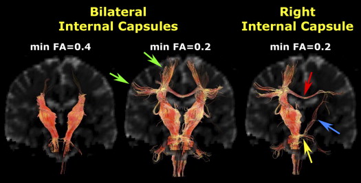
The most widely used of the deterministic streamline tractography methods is known as fiber assignment by continuous tracking (FACT) . Fig. 7 shows an example of FACT-based fiber tracking of ascending and descending tracts that pass through manually placed ROIs in the posterior limbs of the internal capsule. Typical parameters that can be adjusted to alter the results of fiber tracking include the minimum FA threshold to initiate tracking from a voxel, the minimum FA threshold to continue tracking through a voxel, and the maximum turning angle for the streamline between any two voxels. For example, if the streamline encounters a voxel with FA = 0.10 and the minimum threshold to continue tracking is FA = 0.20, then the streamline terminates. Fig. 7 shows the results for fiber tracking with two different FA thresholds: 0.20 and 0.40. Note that the higher threshold traces only the central cores of the tracts, because, as a general rule, the FA is highest near the middle of a tract and falls off at the periphery. Exceptions include regions of complex white matter architecture, where FA is lower because of the presence of crossing fibers. Decreasing the minimum FA threshold for starting or continuing streamlines, or increasing the maximum turning angle, serves to increase the number and length of streamlines identified by the fiber tracking algorithm. The tradeoff, however, is that these changes also increase the number of spurious tracks, ie, streamlines that do not correspond anatomically to actual axonal pathways.