and Yongning He2
(1)
National Institute of Biological Sciences, Beijing, China
(2)
Institute of Biochemistry and Cell Biology, Shanghai Institutes for Biological Sciences, Chinese Academy of Sciences, Shanghai, China
Abstract
Electron tomography (ET) is an emerging electron microscopy (EM) technique for three-dimensional (3D) visualization of molecular arrangements and ultrastructural architectures in organelles, cells, and tissues at 2–10 nm resolution. The 3D tomogram is reconstructed from a series of 2D EM images taken from a single specimen at different projecting orientations. The specimen for ET must be specially prepared to meet the ET imaging requirements, i.e., ultrastructural preservation, specimen thickness, tolerance of electron dose and vacuum, and image contrast. In this chapter, the strategies of specimen preparation of organelles, cells, and tissues and the corresponding EM imaging requirements for ET will be described in detail. In addition, the general procedures tomographic reconstruction and tomogram interpretation will be described.
Key words
Transmission electron microscopyElectron tomographyPlunge freezingHigh-pressure freezingFreeze-substitution fixationOrganelleCellTissue1 Introduction
Biological specimens, such as organelles, cells, and tissues, usually have very complex three-dimensional (3D) architectures. The superposition of 3D structural features into a 2D projection with transmission electron microscopy (TEM) would be ineffective for interpreting the abundant 3D structural information. Electron tomography (ET), an emerging electron microscopy technique suitable for 3D imaging of organelles, cells, and tissues, has largely expanded our biological knowledge from the traditional 2D TEM images to a new level during the past two decades [1–11]. The developments in specimen preparation techniques and EM hardware and software in the past decade have made it possible to visualize the molecular architectures and dynamic cellular events captured in the rapid-frozen specimens at molecular level [12–25], thereby revealing sufficient details for the identification, distribution, and interaction of the target macromolecular complexes. In this chapter, we describe the general technical procedures and methods for performing ET studies of organelles, cells, and tissues.
ET is a computerized reconstruction method for generating a 3D map of a unique specimen from a series of 2D EM projections recorded at different projecting orientations (see Fig. 1). According to the central slice theorem, the Fourier transform (FT) of a 2D projection image of a 3D object is a central slice of the direct FT of the 3D object perpendicular to the projecting direction [26, 27]. If a series of 2D projection images of the 3D object that projected at different directions are collected, their corresponding 2D FT maps (central slices) will constitute a 3D map of the object in Fourier space; thus, the inverse FT of the Fourier space 3D map will result in a real-space reconstructed 3D map of the object (see Fig. 1). Equivalent to the Fourier space approach, tomographic reconstruction can be performed in real space with back projection (see Fig. 1d). In principle, the projection images for ET can be at any random orientations. One of the simplest strategies for collecting projection images is recording a series of projection images by rotating the specimen around a tilt axis at different angles, typically over a tilt range of ±60º or 70º with small increments (1–2º) (see Fig. 1a); these projection images form a single-axis tilt series. However, the slab-like EM specimen cannot be imaged at high angle due to its thickness increasing along the electron beam during rotation. Therefore, single-axis tilt series will have a wedge area without sampling coverage in Fourier space (marked with the gray triangle in Fig. 1b), called “missing wedge,” which will cause non-isotropic resolution in X–Y and elongated distortion in Z-direction of the reconstructed tomogram (as shown in Fig. 1d). To solve the “missing wedge” problem, Radermacher proposed a conical-tilting strategy, which reduces the “missing wedge” to a “missing cone” [28]. Indeed, conical-tilting approach can provide isotropic resolution and reduce the Z-elongation artifacts [29]. However, this approach has disadvantages; it requires all images collected at high-tilt angle, which is difficult to be focused precisely [30]. Another approach to solve the “missing wedge” problem is called the dual-axis tilt series, which collect two single-axis tilt series along two orthogonal axes (simple rotates EM grid by 90º) [30, 31]. Dual-axis approach reduces the “missing wedge” in single-axis case to “missing pyramid,” which can achieve similar coverage in Fourier space as the “missing cone” case. For single-axis tilt series, the un-sampled volume (“missing wedge”) is about 33 % for ±60º and 22 % for ±70º, while in the case of the dual-axis tilt series, the un-sampled volume can be reduced to 16 % for ±60º and 7 % for ±70º [9]; the big differences between the single-axis and dual-axis tomograms are shown in Fig. 7. Actually, dual-axis tomography has become the de facto standard data collection scheme for most tomographic applications.
Fig. 1
Projection acquisition and tomographic reconstruction. (a) Projection. (Left) Tilt series are acquired by tilting the specimen around a tilt axis (here perpendicular to the sheet) at small increments over a limited tilt range. (Center) Projection process of an object made up of four dots with different radii at 0° tilt. (Right) Acquisition of several projections of a tilt series from the object. (b) Assembling the Fourier transform (FT) of the three projections at −45°, 0°, and +45° ((a) Right) in the Fourier space, which is progressively filled as more projections are acquired and their FTs assembled. Afterwards, an inverse FT yields the reconstructed object. The “missing wedge” is marked with gray triangles. (c) The reconstructed object under ideal conditions (sampling and covering). (d) Reconstruction of the object from the tilt series with back projection. From left to right: the reconstruction with tilt series over the range [−50°, +50°] with 1, 3, 5, 15, and 25 projections. The influence of the limited tilt range and the angular sampling are apparent. Reproduced from He and Fernandez [3], with the permission from John Wiley & Sons, Ltd
The concept of ET is not new. The original mathematic idea for tomography was proposed by Rodon in 1917 [26, 27], and the ET approaches were proposed in 1968 [32]. However, due to the technical difficulties, ET was realized in the 1990s after the implementation of automated data collection system in combination with CCD recording system [33–35]. In the past decade, technical improvements have made the cryo-ET tomography possible [36]. Meanwhile, sample preparation has also been improved significantly in recent years, such as plunge freezing [37], high-pressure freezing [38], freeze-substitution fixation [39], frozen-hydrated thin sectioning technique [40–42], and FIB milling [43]. All these methods are towards the faithful preservation of the specimen with high quality, therefore allowing the high-resolution 3D studies with ET. Now, ET is quickly becoming one of the major bio-imaging tools for both cell biology and structural biology [1–11].
In this chapter, we will focus on the general aspects of specimen preparations, electron microscopy imaging and tilt-series acquisition, and 3D reconstruction and interpretation of organelles, cells, and tissues by ET. The technical details of specimen preparation can also be found in other chapters (see Chapters 1–10, 24, 26, and 27). The other 3D electron microscopy approaches, such as phase contrast cryo-tomography (see Chaptes 18), single-particle Cryo-EM (see Chaptes 19), STEM tomography (see Chaptes 27), and FIB-SEM tomography (see Chaptes 24), can be found in other chapters of this book. Since thin sectioning of vitreous thick cells and tissues is still technically demanding, high-pressure freezing/freeze-substitution fixation is the most favorable approach for ET of large objects. In this chapter, we will discuss the ET of thick cells, tissues with high-pressure freezing/freeze-substitution fixation prepared specimens. We will also describe the cryo-ET of the natural thin objects (<0.5–1 μm), such as isolated organelles, thin portions of cells, tiny bacteria, and viruses. We hope that readers can implement their own electron tomography applications by adapting the procedures and techniques described in this chapter.
2 Materials
2.1 Specimen Preparation
1.
High-pressure freezing machine and specimen carriers (e.g., BAL-TEC HPM 010, Wohlwend HPF Compact 01 or 02, Leica HPM 100, Leica EMPACT 2).
2.
Automated freeze-substitution machine (e.g., Leica AFS2, RMC FS-7500).
4.
Plunge freezing system (e.g., FEI Vitrobot, Gatan Cryoplunge).
5.
Carbon coater and carbon rods (e.g., Cressington 208C, Ted Pella, Inc.).
6.
Ultramicrotome UC7/FC7 (Leica Microsystem).
7.
Diamond knife (EMS).
8.
Vaccum oven (20–200 °C).
9.
Dissecting microscope with fiber-optic light source.
10.
2 pairs of 45-degree fine-tipped tweezers (Ted Pella, Inc.).
11.
2 pairs of straight fine-tipped tweezers (Ted Pella, Inc.).
12.
Large forceps for handling cooled cryotubes.
13.
Filter paper (Fisher Scientific, Whatman No. 1).
14.
Paper points (Ted Pella, Inc.).
(a)
HPF specimen carriers (aluminium), type A (0.1 mm/0.2 mm), type B (0.3 mm), or other types (Engineering Office of M. Wohlwend GmbH, Sennwald, Switzerland).
15.
TEM grids:
(a)
Slot grids (EMS; Ted Pella, Inc.).
(b)
200-mesh hexagonal grids (Ted Pella, Inc.; EMS).
(c)
Holey carbon grid: Quantifoil grids R2/1 (EMS), lacey carbon grids (Ted Pella, Inc.), C-flat grids CF-2/1-2C (EMS).
16.
Grid storage box (Ted Pella, Inc.).
17.
PELCO® SynapTek GridStick™ Kit (Ted Pella, Inc.).
18.
50 mL polypropylene centrifuge tubes.
19.
2 mL polypropylene screw cap microtubes (Biologix Research Co.).
20.
2 mL polypropylene snap-lock microtubes (Axygen Scientific).
21.
Glass Pasteur pipettes (Corning).
22.
General transfer plastic pipettes (Ted Pella Inc.).
23.
Liquid nitrogen (LN2).
24.
High-purity ethane.
25.
4 L Dewar for LN2.
26.
1 L wide-mouth LN2 container (e.g., Thermo Scientific).
27.
LN2 workstation.
28.
Resins (e.g., LX-112, Ladd Research).
29.
Micropippetor (1–10 μL) plus tips.
30.
Razor blades or scalpels (EMS).
31.
Crystalline osmium tetroxide (EMS).
32.
10 % glutaraldehyde in acetone (EMS).
33.
Uranyl acetate (EMS).
34.
Formvar 15/95 resin (EMS).
35.
1,2-Dichloroethane (Sigma).
36.
Acetone (>99.7 %).
37.
1-Hexadecene (Sigma).
38.
10 nm colloidal gold solution (Ted Pella, Inc.)
39.
Poly-l-lysine (Ted Pella, Inc.)
40.
BSA (Sigma).
41.
Silicone rubber embedding molds (Ladd Research).
42.
Anhydrous lead citrate Pb(C6H5O7)2.
43.
Lead nitrate Pb(NO3).
44.
Lead acetate Pb(CH3COO)2·3H2O.
45.
Sodium citrate Na3(C6H5O7)·2H2O.
46.
Prepare 1 % OsO4–0.1 % UA fixative in acetone.
(a)
Make 5 % UA in methanol: add 0.1 g uranyl acetate to a 2 mL polypropylene tube. Add 2 mL methanol (precooled on ice) to the tube, and vortex to dissolve completely. Seal the tube and place on ice.
(b)
Add 24.5 mL of acetone (>99.7 %) into a 50 mL polypropylene tube and keep the tube closed on ice.
(c)
Open an ampule with 0.25 g OsO4 (use a rubber ampule breaker or wrap with several layers of paper towels).
(d)
Fetch 0.2–0.3 mL acetone with a glass Pasteur pipette, add to the broken ampule and gently suck in and blow out to dissolve OsO4, and then transfer the solution back to the 50 mL tube. Rinse the ampule with acetone for another 2-3 times, and transfer the solution back to the 50mL tube.
(e)
Add 0.5 mL 5 % UA to the 50 mL tube, and mix well.
(f)
Dispense the 1 % OsO4–0.1 % UA–acetone into 20 cap-numbered 2 mL polypropylene crew cap microtubes by a glass Pasteur pipette (about 1.25 mL per tube, the 1.25 mL position of tube can be pre-labeled out). Cap the tubes immediately and then immerse into LN2 in a 1 L wide-mouth LN2 container by keeping the tubes upright during freezing (let the fixative stay in the bottom).
(g)
Store the frozen 1 % OsO4–0.1 % UA fixative under LN2 until ready to use. Six 2 mL tubes can be stored under LN2 with a 50 mL centrifuge tube with several holes on the top and side (see Fig. 4a).
47.
Prepare 1 % glutaraldehyde fixative in acetone.
(a)
Transfer a 10 mL ampule with 10 % glutaraldehyde in acetone from the −20 °C freezer and warm to 4 °C on ice.
(b)
Prepare 10 cap-numbered 2 mL polypropylene crew cap microtubes.
(c)
Add 1.8 mL pure acetone to each crew cap microtubes at room temperature.
(d)
Open the ampule with 10 % glutaraldehyde in acetone with a rubber ampule breaker or with several layers of paper towels.
(e)
Dispense 0.2 mL of 10 % glutaraldehyde–acetone into each of the 1.8 mL pure acetone-contained microtubes to make 1 % glutaraldehyde–acetone fixative. Cap the tubes immediately and then immerse into LN2 in a 1 L wide-mouth LN2 container by keeping the tubes upright during freezing (let the fixative stay in the bottom). Save the ten 2 mL tubes in two 50 mL centrifuge tubes with several holes under LN2 as storage.
(f)
Dispense the rest 8 mL 10 % glutaraldehyde in acetone into four labeled 2 mL polypropylene screw-capped microtubes (2 mL per tube). Cap the tubes immediately and then immerse into LN2 in a 1 L wide-mouth LN2 container by keeping the tubes upright during freezing (let the fixative stay in the bottom). Save the four tubes in a 50 mL centrifuge tube under LN2 for storage (see Fig. 4a and Note 1).
48.
Prepare 812 resin.
According to the 812 resin product instruction to make mixture A (epoxy + DDSA) and mixture B (epoxy + NMA), here is an example of LX-112 resin (Ladd Research):
(a)
Figure out the weight per epoxide equivalent (WPE) from the product instruction, e.g., WPE = 144; the molecule weight of DDSA (178); and the molecule weight of NMA (266).
(b)
Choose a proper ratio of anhydride/epoxy resin equivalent (the recommended ratio range is 0.6–1.0, for the optimal cutting quality may set the ratio R = 0.63).
(c)
Calculate the weight ratio of DDSA and NMA to LX-112 epoxy resin:
Wdx = R × MW_DDSA/WPE = 0.63 × 266/144 = 1.164.
Wnx = R × MW_NMR/WPE = 0.63 × 178/144 = 0.78.
(d)
Calculate the weights of LX-112, DDSA, and NMA, respectively. Make mixture A (Ta) and mixture B (Tb) as following (aslo see Note 7):
Mixture A: Ta (g) | Mixture B: Tb (g) |
LX-112: Ta/(1 + Wdx) (g) | LX-112: Tb/(1 + Wnx) (g) |
DDSA: Ta × Wdx/(1 + Wdx) (g) | NMA: Tb × Wnx/(1 + Wnx) (g) |
e.g.: medium hardness (Ta:Tb = 1): Ta = Tb = 20 g, Wdx = 1.164, Wnx = 0.78 | |
Mixture A: 20 g | Mixture B: 20 g |
LX-112: 9.24 g | LX-112: 11.24 g |
DDSA: 10.76 g | NMA: 8.76 g |
(e)
Mixture A: weight LX112 (9.24 g) and DDSA (10.76 g) to a 50 mL centrifuge tube. Cap and shake vigorously until thoroughly mixed.
(f)
Mixture B: weight LX112 (11.24 g) and NMA (8.76 g) to a 50 mL centrifuge tube. Cap and shake vigorously until thoroughly mixed.
(g)
Complete LX-112 resin (e.g., 20 g): weight 10 g of mixture A and 10 g of mixture B to a 50 mL centrifuge tube, and cap and shake vigorously until thoroughly mixed.
(h)
Add 0.28 g DMP-30 to the 50 mL tube containing the 20 g complete LX-112 resin. Stir or shake the entire solution for approximately 5 min until thoroughly mixed (if the specimen is incompletely infiltrated, one can use BDMA to replace the DMP-30 [53]).
(i)
Place the 50 mL tube with the complete LX-112 resin in a vacuum oven, evacuating for 20 min to get rid of air bubbles.
(j)
Wrap the tube with aluminium foil, and the resin is ready to use (freshly prepared resin is preferred).
49.
Prepare 3 % uranyl acetate in 70 % methanol.
Add 15 mL ddH2O and 35 mL methanol into a 50 mL tube, cooled on ice. Weight 1.5 g uranyl acetate and add to the 50 mL tube and cap it, and vortex until most uranyl acetate are dissolved at 4 °C. Quickly filter the solution by a syringe filter with 0.2 μm pore size to 4 × 15 mL centrifuge tubes, sealed with Parafilm and wrapped with aluminium foil, and store at 4 °C.
50.
Prepare SATO lead stain solution [56]:
0.20 g anhydrous lead citrate Pb(C6H5O7)2.
0.15 g lead nitrate Pb(NO3).
0.15 g lead acetate Pb(CH3COO)2·3H2O.
1.00 g sodium citrate Na3(C6H5O7)·2H2O.
Weight the above 4 chemicals and add into a 50 mL plastic centrifuge tube, wrapping with aluminium foil. Add 41.0 mL distilled water into the tube, mixed well to a yellowish milky solution. Then the solution is added to 9.0 mL of fresh prepared 1 N NaOH and mixed well until the solution becomes transparent. Quickly filter the solution by a syringe filter with 0.2 μm pore size to 4 × 15 mL centrifuge tubes, sealed with Parafilm and wrapped with aluminum foil, and store at 4 °C (could be stored for a few months).
2.2 Electron Microscopy
1.
Cryo-electron microscope with LaB6 or field emission gun, computer-controlled goniometer, and cryo-stage.
2.
High-tilt tomography holders (maximal tilt angle >60–70° at cryo- and room temperature conditions).
3.
CCD or DDD (e.g.: Direct Electron DE-12, Gantan K2, FEI Falcon) camera for digital imaging.
4.
Cryo-specimen loading station.
5.
Other optional configurations for advanced cryo-ET: multi-specimen autoloader, energy filter, Cs-corrector, and phase plate.
6.
Graphical workstation for image processing and 3D reconstruction (typically CPU >2 GHz, memory >4 GB, storage >200 GB, 3D accelerating graphic card >512 MB).
2.3 Software (See Note 2)
1.
Tilt-series projection image acquisition software.
2.
Tomographic image processing and 3D reconstruction software.
3.
Segmentation and 3D modeling software.
3 Methods
3.1 Specimen Preparation for Electron Tomography
Preparing high-quality biological specimens has been one of the major technical challenges in ET [3, 4, 7, 11]. Unlike the single-particle cryo-EM (see Chaptes 19), ET is mainly dealing with unique molecular architectures and cellular events in cells and tissues, which makes the specimen preparation more technically demanding [3]. Although the conventional EM specimens of cells and tissues prepared by chemical fixation or negative staining (see Chapters 1–4, 11) are informative in many cases, these approaches are usually suffered by artifacts such as flattening, shrinkage, extraction, and aggregation [11, 27, 39, 44]. In order to capture the high-resolution features of the ultrastructure in cells, the rapid freezing techniques (i.e., plunge freezing, high-pressure freezing) are preferred by modern ET (see Chapters 8, 10, 24, and 26). In addition, for achieving accurate interpretation of the ultrastructures, either protein or genetic labeling techniques and the corresponding EM detection techniques are required ([18, 45, 46]; also see Chapters 14–16, 21–26, and 32). To prepare biological specimens suitable for high-quality ET studies, the following factors need to be considered [3]: (1) how to capture the dynamic cellular events rapidly, (2) how to treat water in specimen (to be dehydrated or be frozen hydrated), (3) what is the proper thickness for specimen (usually limited to 200–500 nm), (4) how to improve imaging contrast, and (5) how to identify the target proteins in cells accurately. In this section, we will discuss the challenges and strategies for preparing high-quality specimens for ET (see Figs. 2 and 3).
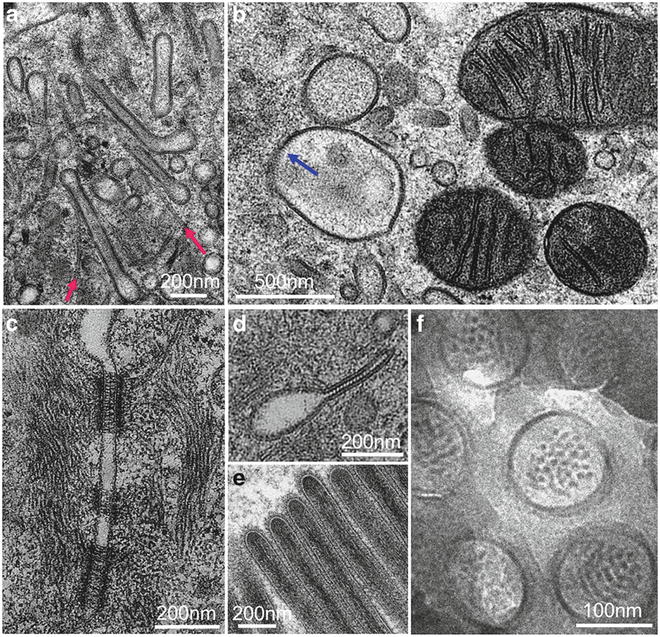
Fig. 2
Strategies and methods for ET specimen preparation. The solid arrows show the specimen preparation methods, while the dash lines represent the EM specimen preparation strategies. Reproduced from He and Fernandez [3], with the permission of John Wiley & Sons, Ltd
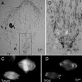
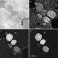
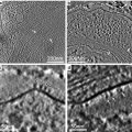
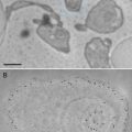
Fig. 3
High-resolution specimens prepared with high-pressure freezing, further processed to dehydrated states by freeze-substitution fixation with 1% OsO4–0.1 %UA in acetone (a–d) or with 0.5 % glutaradehyde–0.01 % tannic acid in acetone (e), or directly thin sectioning at frozen-hydrated state (f). (a–b, d, e, and f) are jejunum epithelial cells from suckling rat. Reproduced from He and Fernandez [3] with the permission from John Wiley & Sons, Ltd. (c) Newborn mice skin, reproduced from He et al. [17], with the permission of the American Association for the Advancement of Science
3.1.1 Biological Experiment Designs
ET of organelles, cells, and tissues can be applied to address many biological questions, e.g., architectures of macromolecular complexes and molecular interactions and dynamic events in physiological or pathological states. Biological experiments must be carefully designed with proper specimen fixation approaches. For example, plunge freezing can be used for capturing the dynamic events in culture cells at certain time points and physiological states, while high-pressure freezing methods are suitable for arresting dynamic events in cells or tissues, such as embryonic development and host–microbe interactions.
3.1.2 Specimen Fixation
High-Pressure Freezing
High-pressure freezing is required for large specimen (e.g., cells or tissues) with thickness up to 200 μM or more [38, 47]. The principle and technical details of high-pressure freezing can be found in Chaptes 8. Here we outline the general procedures for rapid freezing cells and tissues with high-pressure freezing machines (here use BAL-TEC HPM 010 or Wohlwend HPF compact 01 with plate carriers as an example):
1.
Start up the high-pressure freezing machine and wait until the machine is ready for freezing.
2.
Fill the specimen-unloading foam box with LN2.
3.
Pre-clean the specimen carriers (e.g., 0.1 mm/0.2 mm, 0.05 mm/0.25, 0.3 mm aluminium carriers) with acetone and dry in air, and then store them in 1-hexadecene in a 2 mL tube.
4.
Pick a specimen carrier and quickly suck off the excess 1-hexadecene in the carrier with filter paper or Kimwipes, and keep an extremely thin layer of 1-hexadecene on the surface (see Note 3).
5.
Load the cells or tissues into the HPF specimen carriers quickly to minimize the alteration of specimen-required experimental conditions. Make sure the specimen form good contacts with the surface of the carrier.
(a)
(b)
Choose the proper type of carrier for different samples or for different purposes (e.g., frozen-hydrated thin sectioning, FIB milling, freeze-substitution). One should choose the shallowest carrier that matches the specimen and should not overfill the carrier.
6.
Use paper pointer or sharply sliced filter paper to suckle off the excess aqueous medium surrounding the specimen quickly.
7.
Fill 10 μL filler (e.g., 1-hexadecene, n-heptane, 20 % BSA, or other fillers) into the carriers to eliminate air completely.
8.
Take another capping carrier from the 1-hexadecene and cap the specimen without introducing any air bubbles.
9.
Freeze the specimen with high-pressure freezing machine, and make sure the pressure maintenance time (e.g., 300–560 ms) and cooling speed (>−10,000 °C/s) are within the optimal range.
10.
Transfer the frozen specimen immediately to LN2 in the foam box and unload the specimen under LN2.
11.
Open the specimen sandwich by splitting the cap off with a precooled strong forceps or with a precooled blade under LN2. If the filler is 1-hexadecene, use a precooled tweezers to remove the frozen 1-hexadecene from the surface of the specimen gently.
12.
Use precooled forceps to transfer the opened specimen to a 2 mL tube with 1.8 mL frozen freeze-substitution medium (e.g., 1 % OsO4–0.1 % UA or 1 % Glut), and then tighten the screw cap under LN2. (The specimen can also be stored in other specimen storage boxes temporarily and loaded to 2 mL tubes later.)
13.
Store the 2 mL tube in the 1 L wide-mouth LN2 container.
14.
Cover the specimen-unloading box immediately to avoid ice contamination.
15.
Repeat steps 3–11 to freeze the next specimen.
16.
Prepare to shutdown the machine.
Plunge Freezing
Biological samples, such as liposomes, organelles, and small cells, can be vitrified using plunge freezing, a procedure similar to the cryo-EM single particle sample preparation. Plunge freezing can be done with custom-made manually controlled plunge freezer or with automatic plunge freezer, e.g., Vitrobot from FEI (used as an example here). Several types of grids are available for tomographic data collection, for example, Quantifoil grids, lacey carbon grids, and C-flat holey carbon grids. The choice of grids depends on the sample and imaging conditions. Grids with small holes are suitable for small objects such as small vesicles or organelles. For large objects such as cells, grids with large holes would give larger viewing area.
1.
Put grids in a small Petri dish, rinse grids with methanol and air-dry, and then glow discharge for 30 s to 2 min.
3.
Cool down the Vitrobot cup with liquid nitrogen. After approximately 5 min, gently open the valves of the ethane (or ethane/propane mix) tank and fill the central cup of the Vitrobot cup from bottom with a medium flow rate. It may take a couple of minutes before liquid ethane starts forming, and then continue filling until the central cup is full.
4.
Put filter paper on both of the blotting pads in the Vitrobot chamber.
5.
Pick up a grid with the Vitrobot tweezer and loaded onto the Vitrobot plunger.
6.
Mount the Vitrobot cup at the bottom of the Vitrobot.
7.
Set the Vitrobot chamber temperature (e.g., room temperature), humidity (usually 100 %), and blotting time (1–10 s) and offset (1–4 mm) (see Note 5).
8.
Load the sample (1–5 μL) manually with a pipette through a hole on the side of the Vitrobot chamber. For Vitrobot users, sample can also be loaded onto the grid automatically by dipping the grid into a sample tube followed by a quick draining.
9.
Click the start button to start blotting and plunge freezing. After freezing, grids need to be transferred to the grid boxes in the Vitrobot cup with care to avoid ice contamination.
Freeze-Substitution Fixation
1.
2.
Make sure the freeze-substitution chamber is dry, and put the tube holder (here we use a custom-made aluminium block; see Fig. 4b) into the chamber.
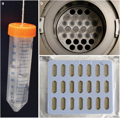
Fig. 4
Custom-made tools for freeze-substitution fixation and an example for resin embedding. (a) A 50 mL conical tube with five holes punched on the cap, and four holes punched on the side near the top, and a string connecting the tube and the cap for 2 mL tubes (with frozen specimens or freeze-substitution medium) storage. (b) Custom-made 30-hole aluminium block for holding the 2 mL tubes for freeze-substitution, usually the screw-capped tube for specimen freeze-substitution fixation and the snap-capped tube for temporary medium exchange. (c) A typical flat mold for embedding of dehydrated specimens, the specimens are usually cut into 0.3–0.5 × 2 mm pieces (0.05–0.3 mm thick)
3.
Add 50 mL pure methanol into the freeze-substitution chamber in the Leica AFS2 machine, and close the chamber by locking the lid.
4.
Fill ~38 L LN2 into the Leica AFS2 LN2 container (fill the LN2 slowly in the beginning to cool down the container).
5.
Program the AFS2 to set a freeze-substitution protocol; here is a typical protocol we preferred (see Note 6):
Step | Temperature | Duration | Notes |
(1) | −90 °C | 30 h | 1 % OsO4–0.1 % UA, or 1 % glutaraldehyde, or other medium. The duration can be changed within the range of 8–72 h |
(2) | −90 °C to −60 °C | 8 h | |
(3) | −60 °C | 24 h | If glutaraldehyde used, this step is required (since glutaraldehyde fixation mainly occurs above -60 °C); If 1% OsO4-0.1% UA used, this step can be reduced to 8 h (since OsO4⧃ fixation is very weak be low -60 °C). Change to other medium if necessary, such as 1% OsO4-0.1% UA or acetone |
(4) | −60 °C to −30 °C | 4 h | |
(5) | −30 °C | 8 h | If OsO4 used, this step is required since OsO4 fixation is mainly occurred above -30 °C |
(6) | −30 °C to −20 °C | 2 h | |
(7) | −20 °C | 8 h | If OsO4 used, this step is required since OsO4 fixation is mainly occurred above -30 °C |
(8) | −20 °C to 4 °C | 2 h | |
(9) | 4 °C | 1 h | 3 × 15 min acetone change to wash away the OsO4 (do not leave the specimen in OsO4 at 4 °C more than 30 min, otherwise the specimen is going to be too dark) |
Warm up to room temperature for resin infiltration (refer to Subheading going to be 3.1.3) | |||
6.
Start the program to cool the chamber to −90 °C, then press “Pause” to stay at −90 °C.
7.
Transfer the 2 mL tube with frozen specimens and freeze-substitution medium by a long forceps from the 1 L wide-mouth LN2 container to the AFS2 specimen chamber, and mount the tubes in holes of the aluminium block.
8.
Lock the lid of the freeze-substitution chamber.
9.
Press “Resume” to resume the freeze-substitution processes.
Chemical Fixation and Progressive Lowering of Temperature
Due to its lower resolution, conventional chemical fixation is not a preferred approach for high-resolution ET [11, 27]. However, for certain cases, the chemical fixation might have some advantages, e.g., conventional chemical fixation combining with immunogold labeling for the identifications and localizations of proteins in fixed cells or tissues [44] and special chemical fixation with negative staining for enhancing the visualization of actin filaments [51]. The details of conventional chemical fixation methods can be found in this book (see Chapters 1, 2, 3).
3.1.3 Resin Infiltration, Embedding, and Polymerization
Resin Infiltration
Step | Medium | Concentration | Duration | Notes |
1 | Resin/acetone | 50 %:50 % | 1.5 h | Prepare 812 resin (refer to Subheading 2.1). 0.5 mL acetone + 0.5 mL LX-112 resin in the 2 mL specimen tube (wrapped with Al foil). Placed on the rotator at 2–4 rpm (same for following steps) |
2 | Resin/acetone | 75 %:25 % | 6–12 h | Leave 0.5 mL 50 %:50 % resin/acetone mixture in the tube, add 0.5 mL resin and mix |
3 | Resin | 100 % | 1 h | Only leave a little resin in the tube, and then add 1 mL fresh resin (fresh prepared or warm up the stock) |
4 | Resin | 100 % | 3 h | Do not suck out the specimen. If the specimen is in suspension or broken into pieces, centrifuge at 1,000 rpm for 1–2 min before sucking out the medium |
5 | Resin | 100 % | 1 h | Ready for embedding |
If specimens are difficult to be completely infiltrated with LX-112 resin, the following protocol can be applied to replace the above steps 1–5: | ||||
1 | Acetone/n-BGE | 50 %:50 % | 15 min | 0.5 mL acetone + 0.5 mL n-BGE in the 2 mL specimen tube (wrapped with Al foil). Placed on the rotator at 2–4 rpm (same for following steps) |
2 | n-BGE | 100 % | 30 min | |
3 | Resin/n-BGE | 50 %:50 % | 1 h | |
4 | Resin/n-BGE | 75 %:25 % | 6–12 h | |
5 | Resin | 100 % | 1 h | |
6 | Resin | 100 % | 3 h
Related posts: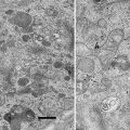 Microwave-Assisted Processing and Embedding for Transmission Electron Microscopy Microwave-Assisted Processing and Embedding for Transmission Electron Microscopy
 Electron Microscopy of Microtubule Cytoskeleton Assembly In Vitro Electron Microscopy of Microtubule Cytoskeleton Assembly In Vitro
 Biological Applications of Energy-Filtered TEM Biological Applications of Energy-Filtered TEM
 Biological Applications of Phase-Contrast Electron Microscopy Biological Applications of Phase-Contrast Electron Microscopy
 Correlative Light and Electron Microscopy Using Immunolabeled Sections Correlative Light and Electron Microscopy Using Immunolabeled Sections
Stay updated, free articles. Join our Telegram channel
Full access? Get Clinical Tree
 Get Clinical Tree app for offline access

| |