and Peta L. Clode1
(1)
Centre for Microscopy, Characterization and Analysis, The University of Western Australia, Crawley, WA, Australia
Abstract
With its low detection limits and the ability to analyze most of the elements in the periodic table, secondary ion mass spectrometry (SIMS) represents one of the most versatile in situ analytical techniques available, and recent developments have resulted in significant advantages for the use of imaging mass spectrometry in biological and biomedical research. Increases in spatial resolution and sensitivity allow detailed interrogation of samples at relevant scales and chemical concentrations. Advances in dynamic SIMS, specifically with the advent of NanoSIMS, now allow the tracking of stable isotopes within biological systems at subcellular length scales, while static SIMS combines subcellular imaging with molecular identification. In this chapter, we present an introduction to the SIMS technique, with particular reference to NanoSIMS, and discuss its application in biological and biomedical research.
Key words
NanoSIMSStable isotopesBiologicalDynamic SIMS1 Introduction
1.1 Secondary Ion Mass Spectrometry
In secondary ion mass spectrometry, a highly energetic ion beam is used to “sputter” material from a sample surface. This primary ion beam impacts the sample surface with energies ranging from a few hundred eV to more than 10 keV, causing a cascade-collision within the top few atomic layers that releases material from the surface. The sputtered material consists of atoms, atom clusters, molecular fragments, and backscattered primary ions. The small proportion of material that is ionized (secondary ions) can be extracted into the mass spectrometer using electrostatic fields. The amount of ionized material is dependent on the ionization efficiency of the element within a specific matrix, and on the primary ion used to sputter the sample, and can vary over many orders of magnitude.
SIMS works in both “static” and “dynamic” regimes depending on the current density of the primary ion beam. In static SIMS, the primary ion dose is typically <1012 ions/cm2, which results in a situation where each impinging primary ion interacts with an essentially pristine area of the sample surface. This leads to the liberation of low-energy secondary ions from within the topmost monolayers only—the surface is not actively eroded by the primary beam—hence, the term “static.” The ejected secondary ions have different velocities depending on their mass, and by measuring the time it takes for the ions to arrive at the detector, it is possible to differentiate between different elements, molecules, and molecular fragments [1]. The pulsed primary ion beam, typically consisting of cluster projectiles such as C60 or Bi300, can be rastered over the sample surface, producing images with lateral resolution up to 100 nm, which record the entire mass spectrum (up to tens of thousands of amu) on each pixel. The technique, however, must trade off lateral resolution for mass resolution and sensitivity and, even under optimum conditions, cannot achieve the mass separation necessary to provide high-precision isotopic analyses. The term “static SIMS” has generally been replaced by “ToF-SIMS” (time-of-flight-SIMS).
Dynamic SIMS, by contrast, uses a high-energy beam that actively erodes the sample surface, producing a higher secondary ion flux but destroying the molecular bonds between the atoms in the sample. Dynamic SIMS typically employs magnetic-sector mass analyzers, where secondary ions are deflected in a magnetic field depending on their mass. Double-focusing mass spectrometers also use an electrostatic sector to filter the secondary ions by kinetic energy either before or after the magnetic-sector. The so-called “sector-field” mass analyzers allow high mass resolution to be achieved with high transmission, providing optimal conditions for high-precision elemental and isotopic analyses. The development of dynamic SIMS over recent years has pushed towards higher sensitivity and better lateral resolution.
While both ToF-SIMS and dynamic SIMS have clear advantages and disadvantages over one another, this paper is primarily concerned with the development and application of high lateral resolution dynamic SIMS for use in biological and biomedical research.
SIMS is a well-established technique in the semiconductor industry, where it has been traditionally used to measure the concentration of dopants and in device failure analysis. The geological community has employed SIMS to quantify trace elements in minerals at concentrations too low for detection by more typical methods such as electron microprobe. It has also proved to be effective in the analysis of stable isotopes in minerals. The lateral resolution, however, has typically been limited to tens of microns because of the geometry of the probe-forming ion optics and as such has attracted little interest from the biological community. As originally proposed by Burns [2], however, there are clear advantages in applying SIMS to biological samples, not least because of the high sensitivity to biologically relevant elements such as C, N, O, S, Na, and K, but also for the potential to detect stable minor isotopes, such as 13C and 15N. Nevertheless, the overriding limitation was the restricted lateral resolution that struggled to differentiate cellular components with any detail.
1.2 NanoSIMS 50
The NanoSIMS 50, conceived by Georges Slodzian [3] and developed by CAMECA (Gennevilliers, France), was designed for imaging with submicron lateral resolution. This is achieved by a novel coaxial lens configuration, which positions the primary probe-forming lens parallel and very close to the sample, allowing the beam to be focused to a very small diameter. The primary ion beam impacts the sample surface at 90°, with the secondary ions extracted back through the same lens assembly. As the coaxial lens uses common focusing optics for both the primary and secondary ion beams, the polarity of the secondary ions must be opposite to that of the primary ions. Currently, two primary ion sources are commercially available for the NanoSIMS: a Cs+ source for the generation of negative secondary ions, which can be focused to a sub-50 nm probe diameter, and a duoplasmatron source that can produce O− and O2 + primary ions, with a smallest beam diameter of about 150 nm. Using the Cs+ primary beam also allows secondary electrons, generated during the sputtering process, to be extracted to a photo multiplier and used for imaging.
High mass resolution is achieved through the use of a double-focusing sector-field spectrometer, consisting of an electrostatic filter (to filter secondary ions according to their kinetic energy) and a magnetic-sector (to separate ions by their mass). The geometry of the mass spectrometer has been optimized to give high transmission and high mass resolution at high lateral resolution, such that a M/ΔM mass resolution of >5,000 with a 100 nm beam diameter is achievable with only an ~25 % loss in transmission. Most significantly, the mass resolution is high enough to separate, for example, 13C from 12C1H on mass 13 and 12C15N from 13C14N on mass 27 (see Fig. 1).
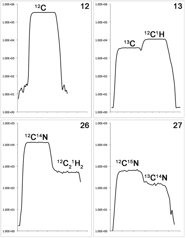
Fig. 1
High mass resolution spectra of peaks on mass 12, 13, 26, and 27. On mass 12, there is only a single peak, 12C− (m = 12.0000). On mass 13, there are two peaks: 13C− (m = 13.0034) and 12C1H− (m = 13.0078), which require an M/ΔM of 2,955 to resolve. The mass resolution is sufficiently high to see a small valley between the two peaks. On mass 26, the dominant peak is 12C14N− (m = 26.0031), but there is a small interference from 12C2 1H2 − (m = 26.0156). Mass 27 has two peaks: 12C15N− (m = 27.0001) and 13C14N− (m = 27.0065), which require an M/ΔM of 4,220 to resolve. The observant reader will have noticed that the sample is significantly enriched in 15N
The secondary ions are focused along the plane of the magnetic-sector where up to seven detectors can be positioned, allowing a large number of mass combinations to be measured. This multicollection capability allows the same microvolume to be sampled on up to seven detectors simultaneously, minimizing the loss of material and increasing throughput. The latest generation of NanoSIMS instruments comes equipped with both electron multipliers (EM) and faraday cup (FC) detectors and electronics that are housed under vacuum and thermally regulated. Imaging is achieved by scanning the focused primary ion beam across the sample, recording the number of incoming ions at the electron multipliers for each pixel of the scan (raster).
1.3 Applications in Biology and Biomedicine
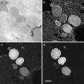
Early dynamic SIMS instruments provided insight into the realm of possibilities available for the biosciences [4]. The advent of high-resolution NanoSIMS resulted in a rapid increase in dynamic SIMS applications throughout the biological and biomedical sciences [5, 6]. For biology, NanoSIMS provides the opportunity to both spatially and temporally study dynamic physiological events—via the detection of either intrinsic or labeled isotopes—at a scale previously unattainable via other SIMS or X-ray detection methods. This subcellular imaging capability, combined with a high sensitivity for biological elements, has resulted in a powerful tool for investigating biological processes at a scale relevant to tissues, cells, and even single microorganisms (see Fig. 2). Areas of research that have utilized NanoSIMS are broad, ranging from medical to environmental applications.
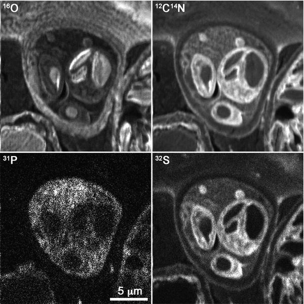
Fig. 2
Secondary ion images of a cell of an Alyssum lesbiacum leaf, obtained by NanoSIMS. The images illustrate the compositional differences between subcellular components
In medicine, NanoSIMS has been successful at locating and measuring heavy metals (e.g., Au and Pt) in cells, introduced via anticancer therapeutics [7, 8], demonstrating the potential in drug delivery studies [9]. Natural iron deposition has also been identified in neural tissues associated with degenerative brain diseases [10, 11]. Changes in Ca distribution have also been identified with secondary degeneration of nerve cells following neurotrauma [12]. The use of labeled isotopes has been used to demonstrate stem cell division and metabolism [13] and the rate of protein turnover in hair cell stereocilia [14].
In environmental studies, metal uptake by plants has been investigated [15–17]. In soil, nutrient cycling has been demonstrated between microbes and plants, using 15N isotopic labels [18]. In fact, NanoSIMS has proved highly adept at deconvoluting the complex relationships between microbes and other organisms. Mapping isotopic labels has shown how bacteria fix nitrogen in bivalves [19] and how marine symbionts transfer nitrogen from seawater to corals [20].
In the last few years, the NanoSIMS has proved to be a revolutionary new tool for microbiologists [21]. The potential to simultaneously determine metabolic activity and identity of naturally occurring microorganisms had been demonstrated using conventional SIMS to analyze indigenous microbes in anoxic marine sediments [22]. Combining fluorescence in situ hybridization (FISH) with SIMS measurements of carbon isotopes found that cell aggregates binding a specific archeal probe were strongly depleted in 13C, indicating a methane-based metabolism. This FISH-SIMS approach is even better suited to NanoSIMS, as it can provide this information at the length-scale of an individual bacterium (~1 μm). Several variations on this approach, termed element-labeled fluorescent in situ hybridization (EL-FISH) or halogen-labeled in situ hybridization (HISH), have been reported [23–26]. But perhaps the most promising approach is catalyzed reporter deposition FISH (CARD-FISH), which deposits high concentrations of fluorine-containing fluorophores in target cells [27].
2 Materials
2.1 Sample Preparation Materials: Chemical Fixation for Nondiffusible Molecules
1.
2.5 % glutaraldehyde in cell-appropriate buffer (PBS, Na-cacodylate, seawater).
2.
Ethanol—50, 70, 90, 100%.
3.
Acetone—100 %.
4.
Epoxy resin (e.g., Araldite 502).
5.
Vacuum system (only needed for large or hard tissues).
6.
Oven at 60 °C.
2.2 Sample Preparation Materials: Cryo-Fixation and Freeze-Substitution for Diffusible Ions
1.
Liquid nitrogen slush system.
2.
Liquid nitrogen.
3.
Acrolein.
4.
Diethyl ether.
5.
Molecular sieve (activated).
6.
Freeze-substitution system (e.g., Leica EM AF2 freeze-substitution unit).
7.
Epoxy resin (e.g., Araldite 502).
8.
Vacuum system (only needed for large or hard tissues).
9.
Oven at 60 °C.
2.3 Sample Sectioning and Mounting
1.
Microtome (e.g., Leica EM UC6 Ultramicrotome).
2.
Glass and/or diamond knives.
3.
10 mm diameter Si wafers or polished metal stubs.
4.
Tetrahydrofuran.
5.
Sputter coater with thickness monitor (e.g., Polaron SC7640 sputter coater).
2.4 Analytical Equipment
1.
NanoSIMS 50 ion microprobe (CAMECA SAS, Gennevilliers, France).
2.
Optical microscope with digital image capture system.
2.5 Data Analysis Software
2.
A spreadsheet application for processing data (e.g., Microsoft Excel).
3 Methods
3.1 Sample Preparation
3.1.1 Chemical Processing
Ideally samples should be less than 2 mm3, otherwise vacuum treatment may be required, especially for hard tissues such as plant leaves and stems.
1.
Samples should be fixed in 2.5 % glutaraldehyde in a suitable buffer for at least 1 h to cross-link and fix the cellular material [28].
2.
Progressively dehydrate samples in a graded ethanol series, beginning at 50 % and finishing at 100 %, followed by 100 % acetone. Each step should be 10 min (longer for larger tissues).
3.
Incrementally infiltrate with resin. Start with resin:acetone mixtures at 1:2, then 2:1, and finally 100 % resin, for 1 h each (see Note 2).
4.
Mount samples in 100 % resin and cure as per resin requirements (60 °C for 36 h for Araldite 502).
3.1.2 Cryo-Processing
For the analysis of diffusible ions, samples can be prepared according to Marshall [29]. All liquids (including resin components) and solvents must be anhydrous to prevent redistribution or loss of diffusible ions (see Note 3). A typical substitution protocol suitable for retaining diffusible ions is given in Table 1. Samples must be rapidly frozen to achieve optimal cellular freezing rates and to limit ice crystal formation [30].
Table 1
Freeze-substitution protocol suitable for retaining diffusible ions when 10% acrolein in diethyl ether with molecular sieve is used as the substitution medium
Temperature ( °C) | −100 | −90 | −70 | −20 | 0 |
Time (h) | 24 | 168 | 336 | 24 | Hold |
1.
When using liquid nitrogen slush, samples must simply be rapidly plunged into liquid nitrogen slush (see Note 4). If necessary, they can be stored in liquid nitrogen until freeze-substitution is performed.
2.
For freeze-substitution, frozen samples are transferred (without warming) to a cryovial containing 10 % acrolein in diethyl ether mixture with activated molecular sieve. The solution should be maintained at <−120 °C in a bath of liquid nitrogen to avoid sample warming.
3.
Over the following 3 weeks, samples should be slowly warmed. As ice is not very soluble in ether, long substitution times are required [30].
4.
Once substitution is complete, bring the samples to room temperature and rinse in diethyl ether.
5.
Infiltrate with resin incrementally, with resin:ether mixtures starting at 1:2, then 2:1, and finally 100 % resin, for 1 h each (see Note 2).
6.
Mount samples in 100 % resin and cure as per resin requirements (60 °C for 36 h for Araldite 502).
7.
Samples should be stored in a desiccator to avoid absorption of water and possible movement of ions.
3.1.3 Sample Sectioning and Mounting
1.
Resin blocks should be trimmed to achieve the desired sample orientation [31]. For high-quality sections, a diamond knife should be used, but glass is also usually sufficient.
2.
Sections are cut using a microtome to a thickness of 750 nm–1 μm.
3.
Sections should be mounted on an appropriate substrate (see Note 5) using either water (for chemically processed material) or anhydrous tetrahydrofuran (for freeze-substituted material) to disperse the section on the mount.
4.
Images of the mounted sections must be recorded with a reflected light microscope, as these are essential for navigating in the NanoSIMS and locating regions of interest (see Fig. 3).
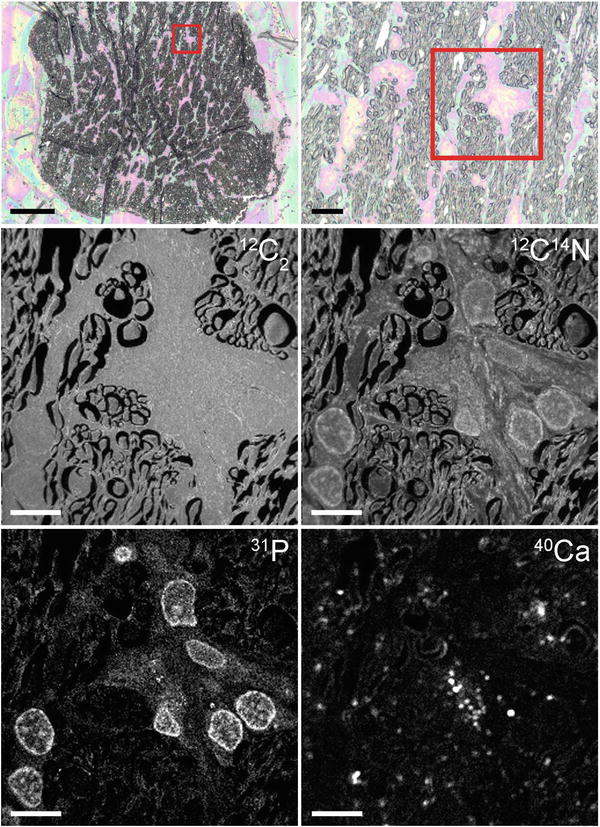
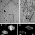
Fig. 3
A 1-μm-thick cross section of the optic nerve tissue after partial injury, prepared using cryo-processing techniques. The top two panels show optical images obtained with a standard reflected light microscope (scale bars = 100 μm and 20 μm, respectively). The red box marks the area imaged using the NanoSIMS. The 12C2 − image reveals the ubiquitous presence of C; the 26CN− image clearly shows the cell morphology—axons and glia; the 31P− image highlights the nuclei of the glial cells; and the 40Ca+ image reveals the location of Ca2+ microdomains within the tissue (scale bars on NanoSIMS images = 10 μm). These images were obtained using both the Cs+ and O− primary ions sources (Color figure online)
3.2 Data Acquisition
This section outlines the procedures for the acquisition of images of biological samples using the NanoSIMS 50 ion microprobe.
1.
Check if the vacuum throughout the NanoSIMS is good and if the source chamber and multicollection chamber valves are open.
2.
Check if the cooling water flow is sufficient.
3.
Turn on the HV button on the keyboard, and load the preset files.
3.2.1 Primary Beam Tuning
The choice of a Cs+ or O− primary beam is determined by the polarity of the secondary ions to be analyzed (see Note 7).
Tuning the Cs+ Primary Ion Beam
1.
To start the Cs+ source, type the desired values for the ionizer and reservoir into the source software window. The HV should be set to 8,000 V. The source takes about 20 min to start up but will continue to warm up over the next several hours (see Note 8). To obtain the best stability, it is advisable to set the automatic start-up to initiate about 2 h before the source is needed.
2.
3.
Check the primary beam reaching the sample either by measuring the Fco value or by checking the signal on the secondary electron (SE) detector.
4.
 Microwave-Assisted Processing and Embedding for Transmission Electron Microscopy
 Electron Microscopy of Microtubule Cytoskeleton Assembly In Vitro
 Biological Applications of Energy-Filtered TEM
 Freeze Fracture and Freeze Etching
 Correlative Light and Electron Microscopy Using Immunolabeled Sections
 X-Ray Microanalysis in the Scanning Electron Microscope


Using the Si grid standard, obtain an SE image using the real-time imaging mode (RTI) and the D1 aperture set to 300 μm (see Note 11). Adjust the sample height, z, to focus the image for the value of the primary focusing lens (EOP) that is normally used (see Note 12).
Related posts:
Microwave-Assisted Processing and Embedding for Transmission Electron Microscopy
Electron Microscopy of Microtubule Cytoskeleton Assembly In Vitro
Biological Applications of Energy-Filtered TEM
Freeze Fracture and Freeze Etching
Correlative Light and Electron Microscopy Using Immunolabeled Sections
Stay updated, free articles. Join our Telegram channel
Full access? Get Clinical Tree
