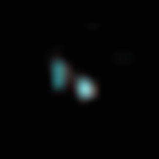
Quantitation of Chromosome Damage by Imaging Flow Cytometry

Fig. 1

Example of an object (#1605) in each of the collected channels (channel 5 bright field, channel 1 Hoechst 33258 and channel 2 PNA probe) as well as a composite view of channels 1 and 2 overlayed

Create a plot of Intensity of channel 1 (Hoechst 33258) versus Intensity of channel 2 (PNA), where the Intensity feature is the sum of the background subtracted pixel values within the masked area of the image. In this way you can select for two-colour positive populations (see Fig. 2). Note that cells can also be identified and rejected (identified as “cells” in Fig. 2).

Fig. 2

Scatterplot of Intensity of channel 1 (Hoechst 33258) versus Intensity of channel 2 (PNA probe) to identify two-colour positive population “2colourPos”. Noted on the plot is a population of “cells” which appear to be intact. Also shown is a population identified as “Reject-01” with some example objects to the left

Visually investigate identified populations to ensure that gates are including objects of interest without including too many unwanted objects (see Fig. 3).

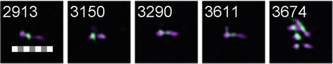
Fig. 3

Selection of objects from the “2colourPos” population with a scale bar of 7 μm for reference. Note that some of the objects appear to be aggregates of multiple chromosomes (object #3674)

10.

Based on the two-color positive population, create a new scatterplot of the Contrast of channel 5 (bright field) versus the Contrast of channel 1 (Hoechst 33258), where Contrast measures the sharpness quality of an image, to select a sub-selection of objects with good contrast (see Fig. 4, Note 30 ).

Fig. 4

Based on the two-colour positive chromosome population identified in Fig. 2, plot Contrast of channel 5 (bright field) versus the Contrast of channel 1 (Hoechst 33258) to identify objects with good contrast. Examples of objects in each of the “good Contrast” and “Reject-02” region are shown alongside the gates

11.

Again, visually inspect the populations to verify the stringency of the gating strategy. Figure 4 shows a selection of objects from each gate (Reject-02 and goodContrast) and illustrates the difference in image quality.

12.

From the goodContrast population, create a scatterplot of the Area of channel 2 (PNA probe), where Area is equal to the number of microns squared in a mask, versus the Intensity of channel 2 to remove objects that have too much PNA probe (see Fig. 5, Note 31 ).

Fig. 5

Scatterplot of the Area of channel 2 (PNA probe) versus the Intensity of channel 2

13.

From the centArea population created in step 12, create a scatterplot of the Area of channel 5 (bright field) versus the Aspect Ratio Intensity, defined to be the ratio between the intensity weighted minor axis of the image divided by the intensity weighted major axis of the image, of channel 6 (side scatter), to remove objects that appear to be doublets (Reject-04), leaving a population of apparently single chromosomes (Singles) (see Fig. 6).

Fig. 6

Scatter plot of the Area of channel 5 (bright field) versus the Aspect Ratio Intensity of channel 6 (side scatter). Two populations are shown, one of objects considered to be single chromosomes “singles,” and another of objects considered to have multiple chromosomes or aggregates “Reject-04.” Examples of objects in each population are shown adjacent to the respective gates

14.

To quantify the chromosome damage, follow steps 15–17; iterate as required to fine tune the masking strategy.

15.

Create a spot mask based on the centromere signal as shown in Fig. 7 (see Note 32 ).

Fig. 7

Masking of PNA probe signal (see Note 32 )

16.

Plot a histogram of spot counts based on the mask created in step 15 (see Fig. 8).

Fig. 8

Histogram of Spot counts. These gates represent monocentric (1-cent) and dicentric (2-centric) chromosomes

17.

Create gates on the histogram bins for chromosomes with each number of centromeres (spots). Check each of these gates to see if the included objects are good representations of chromosomes with the specified number of centromeres (see Note 33 ).

4 Notes

If a 405 nm laser is not available, the method can be adapted for use with a different laser and an alternative DNA stain, i.e., propidium iodide on the 658 nm laser.

Make fresh on the first day of the experiment. For a 70 mL final volume, start with 56.8 mL RPMI 1640 media and add 0.7 mL l-Glutamine-Penicillin-Streptomycin, 10.5 mL heat-inactivated FBS, 1.26 mL PHA, and 0.7 mL colcemid. Let warm in an incubator until needed.

pH 7.4 in ddH₂O and filter sterile. Can be stored at RT for up to a year.

pH 7.4 in ddH₂O and filter (0.2 μm) and store at RT for up to several months.

Only gold members can continue reading. Log In or Register to continue