, Alexander A. Gall2 and Luda S. Shlyakhtenko1
(1)
Department of Pharmaceutical Sciences, University of Nebraska Medical Center, Omaha, NE, USA
(2)
Cepheid, Bothell, WA, USA
Abstract
This article describes sample preparation techniques for AFM imaging of DNA and protein–DNA complexes. The approach is based on chemical functionalization of the mica surface with aminopropyl silatrane (APS) to yield an APS-mica surface. This surface binds nucleic acids and nucleoprotein complexes in a wide range of ionic strengths, in the absence of divalent cations, and in a broad range of pH. The chapter describes the methodologies for the preparation of APS-mica surfaces and the preparation of samples for AFM imaging. The protocol for synthesis and purification of APS is also provided. The AFM applications are illustrated with examples of images of DNA and protein–DNA complexes.
Key words
Atomic force microscopyAFMMica functionalizationSurface chemistrySilanesSilatranesDNA structure and dynamicsProtein–DNA complexes1 Introduction
1.1 AFM Basics
The prototype scanning tunneling microscope (STM) instrument was conceived by Binnig and Rohrer [1, 2], an invention for which the authors were awarded the 1986 Nobel Prize in Physics. The atomic force microscope (AFM) was invented in 1986 [3], and commercial instruments became available to the biological community shortly thereafter. A schematic illustrating the principles of the AFM operation is shown in Fig. 1. A sharp stylus (AFM tip shown as a triangle) reads the profile of the sample (shown as a bumpy profile) by scanning over the sample. The tip is attached to a cantilever that works as a spring pressing the tip against the sample to reproduce the surface profile. The vertical position of the tip is measured by a laser light reflected from the cantilever to the position-sensitive photodetector (PSD). According to this scheme, no special contrasting sample is needed for AFM imaging. Additionally, scanning can be performed in any media at ambient conditions, including physiological conditions, making AFM very valuable for biological applications.
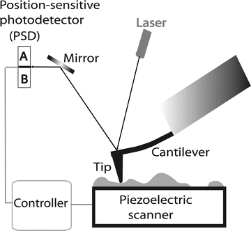
Fig. 1
Schematic explaining the principles of AFM. The position of the tip relative to the sample is controlled by a piezoelectric scanner. The vertical displacement of the tip during scanning is detected using the optical lever principle, in which the position of the light spot on the PSD is measured
AFM instruments include a number of important features that enable the production of high-resolution images. First, the position of the sample relative to the tip is controlled by the scanner with an accuracy of less than 1 nm. Second, the tip can be atomically sharp. Third, the displacement of the tip relative to the surface is determined with sub-nanometer accuracy. These three major features provide the foundation for AFM’s capability of producing topographic images with atomic accuracy. Atomic resolution was achieved with AFM in an early paper [4] in which the atomic-scale periodicities of calcite as well as the expected relative positions of the atoms within each unit cell were obtained. This capability of achieving atomic level resolution was further exemplified by a recent publication reporting differences of 74 pm in lengths of covalent single and double bonds [5]. The authors estimate that the developed AFM methodology (the instrument operated in a noncontact mode at cryogenic temperature, 5 K) is capable of measuring the bond length difference down to 30 pm.
Figure 2 illustrates the major operating modes of AFM. The operating mode corresponding to the attraction part of the tip–sample interaction potential is termed noncontact mode (NC-AFM). After passing the minimum on the potential curve, the repulsion interaction rises steeply, achieving large positive values in a very short range of the tip–sample distances. This scanning regime is termed contact mode. In this regime, the tip strongly interacts with the surface; therefore, in the contact mode AFM does not allow for obtaining reliable and robust imaging biological samples. Importantly, damage or deformation of soft biological samples can be made by the tip during the approach or scanning process.
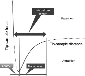
Fig. 2
Schematic explaining the different modes of AFM operation. The curve in the schematic shows the change of the tip–sample interaction energy dependent on the distance between the apex of the tip and the sample
The alternating contact (AC) AFM mode is efficient in numerous biological applications and was initially proposed in [6]. In this mode, the AFM tip oscillates with a frequency much faster than the scanning frequency and is in contact with the sample during a short period of time. For typical AFM experiments in air, the tip oscillates with ~100 KHz, while the scanning frequency is 2–4 Hz. This mode dramatically decreases tip deformation and dragging effects. Another term for AC mode is tapping mode [7]; but the name has been trademarked by the AFM manufacturer, Veeco. Other manufacturers use AC mode or intermediate or intermittent contact mode (IC mode). Schematically, the range of operation of the AC/IC/TM mode is illustrated in Fig. 2 with a thick horizontal double arrow.
In contact mode, the tip–sample distance is maintained by measuring the deflection of the tip cantilever determined by van der Waals repulsion forces. However, the detection principle for the intermediate mode is different. In AC/IC/TM-AFM, a cantilever is deliberately vibrated at the frequency close to the cantilever resonance frequency by a piezoelectric modulator with a very small amplitude. As the tip approaches a surface, the van der Waals attractive force between the tip and the sample changes both the amplitude and the phase of the cantilever vibration [8]. These changes are monitored by a Z-servo system feedback loop to control the tip–sample distance. The ability of the AC/IC/TM mode to image biological samples gently is the primary attractive feature of this operating mode. The paragraphs below briefly describe a few examples in which AC/IC/TM-AFM was applied to image DNA and protein–DNA complexes.
1.2 AFM for Imaging of Protein–DNA Complexes
Figure 3a shows an AFM image of supercoiled DNA with a plectonemic morphology formed by interwound DNA strands of a circular DNA molecule. The next frame (Fig. 3b) shows the complex of DNA with the site-specific binding protein SfiI, as described in refs. [9, 10]. This is a restriction enzyme that cleaves DNA when it binds two recognition sites on DNA forming a synaptic complex, as shown schematically below the image. The images contain looped complexes directly proving the existence of synaptic complexes (Mg2+ cations were replaced with Ca2+ cations to prevent DNA cleavage). Protein binding specificity was confirmed by the length measurements of multiple images. Schematic in (b) illustrates the positions of binding sites (squares) on the DNA substrate.
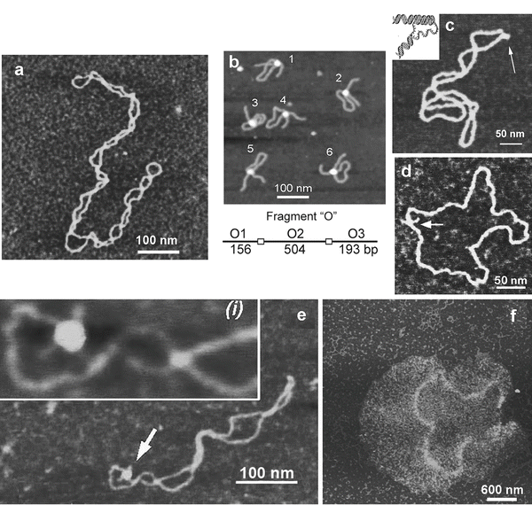
Fig. 3
A set of AFM images of various samples. Plate (a) shows the AFM image of supercoiled plasmid DNA. Plate (b) shows AFM images of complexes of DNA with SfiI restriction enzyme. The schematic in (b) explains the design of the DNA construct; positions of the SfiI binding sites are indicated with squares and the numbers are shown in base pairs (bp). More information and animated images can be found in ref. [55]. The figure was reproduced from Lushnikov [55] with the permission of the American Chemical Society. Plate (c) shows the image of plasmid DNA with H-form DNA appearing as a clear-cut protrusion on the image. pCW2966 contains a 46 bp mirror repeat forming H-DNA at acidic pH. A sharp kink at the base of the thick protrusion is indicated with an arrow. The inset shows the schematic for H-DNA structure. More information and animated images can be found in [12]. The figure was reproduced from Tiner et al. [12], with the permission of Elsevier. Plate (d) shows the image of circular pUC8F14C plasmid DNA containing a 106 bp inverted repeat forming cruciforms under appropriate supercoiling density. DNA with the cruciform protrusion is indicated with an arrow. Image (e) demonstrates the formation of complexes of the same plasmid DNA with RuvA protein (indicated with an arrow). Inset (i) is the higher-resolution image of the DNA segment with the bound protein. More information can be found in ref. [15]. The figure was reproduced from Shlyakhtenko et al. [15] with the permission from Elsevier. The images were acquired in air with MultiMode AFM operated with NanoScope IIId and IV controllers (Veeco)
An intramolecular DNA triplex or H-DNA formed by homopurine–homopyrimidine (Pu·Py) tracts is a biologically important alternative DNA structure [11]. Structural studies of intramolecular triplexes are instrumental in understanding the mechanism of how H-DNA is involved in genetic processes. The challenge in imaging H-DNA is the requirement of low pH. This requirement was met in a publication [12] in which the functionalized mica approach was implemented. A high-resolution AFM image of pUC19 plasmid with a 46 bp long purine–pyrimidine repeat prepared at acidic pH is shown in Fig. 3d. A distinct feature of the molecules prepared at acidic pH is the formation of a clear kink with a short protrusion indicated by an arrow. The formation of a sharp kink is fully consistent with the model of an intramolecular DNA triplex [11, 13] shown schematically in Fig. 3c. The same technique was instrumental in detecting the H-DNA conformation in long imperfect Py–Pu inserts [14].
Figure 3d illustrates the ability of AFM to image another type of transient DNA conformation, cruciforms. Negative DNA supercoiling is required for cruciform stabilization. The cruciform appears on the AFM image as a clear-cut extrusion as indicated with an arrow. The sizes of the arms for extended extrusions are 15–20 nm, in full agreement with the expected length of the hairpins containing 53 bp (18 nm for B-helix DNA geometry). The identification of two classes of cruciforms, discovered by AFM imaging, led to the hypothesis of a novel regulatory role of cruciforms in global DNA dynamics [15]. Both alternative DNA structures, cruciforms and H-DNA, are involved in the regulation of DNA transcription; therefore, the ability of AFM to image alternative DNA structures makes AFM a very valuable tool in the field of molecular and structural genetics.
Figure 3e shows an AFM image of the complex formed by a cruciform with RuvA protein [15]. RuvA is the key protein involved in DNA homologous recombination that recognizes four-way DNA junctions, such as cruciforms. AFM confirmed this binding specificity demonstrating that after binding to the cruciform, the protein unfolds it and keeps the cruciform in unfolded conformation. Based on these findings the authors proposed a novel regulatory mechanism for DNA recombination [15].
The ability of AFM to image a large DNA assembly termed kinetoplast DNA (kDNA), in addition to individual DNA molecules, was demonstrated in [16] (see Fig. 3f ). This natively existing large and fragile molecular assembly consists of several thousand DNA circles of approximately 2 kb (minicircles) and a few dozen much larger DNA molecules, termed macrocircles, interlocked into a network. The gentle operating capabilities of AFM, combined with appropriate sample preparation procedures, were two critical issues enabling the observation of intact fragile biological systems such as kDNA [16].
1.3 Time-Lapse AFM Imaging of Protein–DNA Complexes
One of the important features of AFM is the ability to scan samples in aqueous solutions. This mode of AFM imaging is appealing for two major reasons. First, imaging of the fully hydrated sample eliminates potential problems inherent with sample drying. Second, imaging in liquid allows for time-lapse visualization of sample dynamics and interactions. Importantly, due to AFM resolution at the nanometer scale, dynamics are observed at the nanoscale level. Various protein–DNA systems were analyzed with the time-lapse AFM that were reviewed in refs. [17–19]; see also references therein. The drawback of AFM time-lapse studies is the slow (minute-scale) data acquisition rate of a conventional AFM instrument, so most system dynamics remain undetectable. Ando’s group has developed a high-speed AFM (HS-AFM) instrument operating almost 1,000 times faster and capable of acquiring data with a sub-second rate [20–22]. With this instrument, Ando’s group was able to visualize the dynamics of individual myosin molecules with a 100 ms temporal resolution [21, 22]. HS-AFM was instrumental in the analysis, performed by our group and others, of various protein–DNA complexes [23–27]. Its application to understand the mechanism of interactions of site-specific binding proteins with DNA is illustrated in Fig. 4. This figure shows four frames (out of several hundred) spanning over 20 s in which the process of searching specific sites by site-specific EcoRII protein was directly visualized [28]. The initial state (5 s) is a complex with a small loop that gradually increases over time (10 s). After 15 s, the protein stops moving and binds to another specific DNA site, as indicated by DNA length measurements. The change in the loop length occurs over a period of about 10 s, covering a distance of about 300 bp (102 nm) until the EcoRII complex stops at another recognition site, which corresponds to a rate of about 30 bp/s (10.2 nm/s). These data suggest that EcoRII binds to one recognition site and searches for another site by threading the DNA filament through the complex until the enzyme finds the second recognition site, upon which it forms a stable synaptic complex.
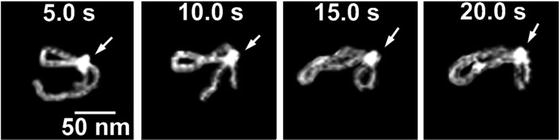
Fig. 4
EcoRII translocation process analyzed by high-speed AFM. Four frames out of 40 frames total were taken over a time period of 20 s measured in 0.5 s intervals. In the first frame (5 s) the looped structure is formed, stabilized by the protein (indicated with an arrow) bound to two specific sites on the DNA. The following frames illustrate sliding of the protein along the DNA strand, leading to an increase in the loop size. The final image (20 s), in which a large loop is formed, corresponds to binding of the protein to two distant binding sites on the DNA substrate. More information and animated images can be found in ref. [28]. The modified figure was reproduced from Gilmore et al. [28], with the permission of the American Chemical Society
1.4 Sample Preparation Approaches for AFM of DNA and Protein–DNA Complexes
The scanning tip can move or even sweep the samples that are weakly bound to the surface. Ignoring the sweeping effect led to a number of scanning artifacts identified in early attempts to image DNA with scanning tunneling microscope (STM), a predecessor of AFM [29–32]. Therefore, the sample preparation procedure was emphasized in AFM studies of DNA and protein–DNA complexes. The first results revealing reliable AFM images of long DNA molecules were reported in the early 1990s when a number of sample preparation methods were developed [33, 34]. The laboratory of C. Bustamante [34] implemented the method of mica cationic treatment [35]. In this approach, the mica surface is treated with Mg2+ to increase the affinity of the negatively charged mica surface to DNA. Other metal cations such as Co2+, La3+, and Zr4+ can be used for mica pretreatment to obtain images of DNA [36]. Later, experiments showed that pretreatment of mica with cations was not necessary [37–40], as DNA adheres if Mg2+ cations are present in the buffer. In the laboratory of Z. Shao, an approach utilizing a modification of the well-known electron microscopic procedure for imaging DNA was developed [41, 42]. This method involves spreading DNA onto a carbon-coated mica substrate following cytochrome c denaturation at the air–water interface. Among these methods, the cation-assisted technique has become the most widely used due to the simplicity of sample preparation. However, the requirement for multivalent cations is mandatory and therefore limits the range of experimental conditions to buffers with a defined concentration of cations. Alternatives to these techniques were methods utilizing mica functionalization (reviewed in refs. [19, 43–45]). A weak cationic surface is obtained if (3-aminopropyl)triethoxysilane (APTES) is used to functionalize the mica surface with amino groups (AP-mica). As a result, functionalized surfaces remain positively charged at pH below pK a values (pK a = 10.4) and are capable of binding to negatively charged DNA in the pH range of stable DNA duplexes. Hydrolysis and aggregation of APTES is a complication associated with this technique.
An alternative to this technique is a more hydrolytically stable silatrane reagent, 1-(3-aminopropyl) silatrane (APS). Slow hydrolysis of the silatrane moiety allows avoidance of clumping and enables a smooth modification of the surface with amino groups achieving results similar to APTES vapor treatment. The schematics for the APS chemical formula and its reaction with the mica surface are shown in Fig. 5. The reaction with the surface (Fig. 5a) proceeds through several steps with eventual loss of the triethanolamine molecule and covalent attachment of the 3-aminopropyl siloxane group to the mica. The silatrane can be bound to several adjacent OH groups and these arrangements are shown in Fig. 5b. Both AP-mica and APS-mica methods are robust and work reproducibly in various topographic studies involving DNA [10, 12, 14, 44, 46–55]. Additionally, the APS-mica methodology works reliably for force spectroscopy AFM applications [56–60]. The sections below provide specific details related to the preparation of APS-mica surfaces for AFM imaging, including the procedure for the synthesis of the APS reagent.
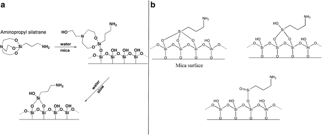
Fig. 5
The reaction of aminopropyl silatrane (APS) with silicon surfaces. (a) Schematic for the reaction of APS with the hydroxyl groups (OH groups) on silicon surfaces. The OH groups on the mica surface formed spontaneously after cleavage. Initial and final stages of the reaction are shown. Note the last stage, exposure of APS-functionalized mica to water, leads to dissociation of triethanolamine yielding the stable product. (b) illustrates the reaction of APS with three, two, and single OH groups (from left to right). Mica contains Al atoms as shown in this scheme
2 Materials
2.1 General Equipment, Solutions, and Supplies
1.
A vacuum cabinet or desiccator for storing samples. A Gravity Convention Utility Oven (VWR) is recommended.
2.
Plastic tubes, 15 mL.
3.
Eppendorf tubes, 1.5 mL.
4.
Plastic cuvettes.
5.
Scissors.
6.
Razor blade.
7.
2 L glass desiccators and vacuum line (50 mmHg is sufficient).
8.
Pipettes with plastic tips for rinsing the samples.
9.
Tweezers.
10.
Gas tank with clean argon gas. Nitrogen gas can be used as well.
11.
Mica substrate. Any type of commercially available mica sheets (green or ruby mica) can be used. Asheville-Schoonmaker Mica Co (Newport News, VA) supplies thick and large (more than 5 cm× 7 cm) sheets (Grade 1) suitable for making substrates of different thickness and size.
12.
Deionized water filtered through 0.2 μm filter for mica functionalization and AFM sample preparation.
13.
Solution of sodium hydroxide in methanol (2 mg/mL).
14.
AFM tips. For imaging in air, any type of tip with a spring constant of approximately 40 N/m and a resonance frequency between 300 and 340 kHz can be used. For example, Olympus silicon probes (Asylum Research, Santa Barbara, CA), with a spring constant of 40 N/m and a 300 kHz resonance frequency in air, work reliably in the tapping/oscillating mode for imaging in air. Probes with similar characteristics are currently manufactured by a large number of other vendors.
15.
For imaging in liquid with a regular AFM, Si3N4, 100-μm-long probes (SNL, Bruker Nano/Veeco, Santa Barbara, CA) with a spring constant of approximately 0.06 N/m and a resonance frequency around 7–10 kHz were used. Tips with similar characteristics from other vendors are available.
16.
AFM instrument. Many instruments from different vendors are currently available. The authors used MM AFM (Bruker Nano, Santa Barbara, CA) for years; therefore, the instrument-related specifics are described for this particular instrument.
3 Methods
3.1 Synthesis of Aminopropyl Silatrane (APS)
The procedure described below is a modified version of our previously published method [45]. We tested and verified that sodium hydroxide can be used as a catalyst instead of the previously recommended sodium metal. We also found that reproducibility and chance of crystallization after reaction completion substantially improve when precise stoichiometric amounts of triethanolamine and (3-aminopropyl)triethoxysilane are used. For this purpose, we recommend using a precision balance rather than graduated cylinders for measuring the volumes of these liquid reagents. The reaction is essentially quantitative and is described by the schematic in Fig. 5a (see Notes 1 and 2 for additional information).
1.
Prepare the 2 mg/mL by adding sodium hydroxide granules to the calculated amount of methanol and stirring until all sodium hydroxide is completely dissolved. Sonication or moderate heat can accelerate the process (Caution: sodium hydroxide solid and solutions can cause burns to the eyes and skin. Do not heat a closed vial.).
2.
 Microwave-Assisted Processing and Embedding for Transmission Electron Microscopy
 Electron Microscopy of Microtubule Cytoskeleton Assembly In Vitro
 Biological Applications of Energy-Filtered TEM
 Biological Applications of Phase-Contrast Electron Microscopy
 Correlative Light and Electron Microscopy Using Immunolabeled Sections
 X-Ray Microanalysis in the Scanning Electron Microscope


Add triethanolamine (14.92 g, 0.1 M) to a 250 mL round-bottom flask followed by 2 mL of sodium hydroxide solution in methanol (2 mg/mL). A precise equivalent amount of (3-aminopropyl)triethoxysilane (APTES; 22.14 g, 0.1 M) is measured in a separate flask and added to the reaction mixture. Complete transfer of the reagent is assured by washing the flask with two portions of methanol (2 × 10 mL) and adding the methanol washes to the reaction mixture.
Related posts:
Microwave-Assisted Processing and Embedding for Transmission Electron Microscopy
Electron Microscopy of Microtubule Cytoskeleton Assembly In Vitro
Biological Applications of Energy-Filtered TEM
Biological Applications of Phase-Contrast Electron Microscopy
Correlative Light and Electron Microscopy Using Immunolabeled Sections
Stay updated, free articles. Join our Telegram channel
Full access? Get Clinical Tree
