8 Computed Tomography
In the multislice spiral technique, computed tomography (CT) acquires nearly isotropic voxels. With volume acquisition by means of thin slices, between 0.5 and 1.0mm of thickness, the process of scanning the hand is primarily necessary to only one plane: the axial plane on the carpus, the oblique-sagittal plane on the scaphoid, and the sagittal plane on the metacarpus and the fingers. Multiplanar reconstruction (MPR) slices in all other planes as well, as three-dimensional surface views, can be calculated from the dataset. Computed tomography provides high-resolution sectional views of the skeleton of the hand that display the fine trabecular bone structure, the compact bone, and the subchondral bone plate in an edge-enhanced reconstruction algorithm. The main indications for CT are intra-articular radius fractures and fractures of the scaphoid and uni- or multilocular fractures of the other carpal bones, especially when complex trauma is involved. Other important indications are evaluation of scaphoid nonunion and identification of initial stages of osteoarthritis.
General Principle of CT
During the scanning process, the x-ray tube (the radiation source) and the detectors (the image-recording system) opposite it rotate around the patient in the same direction. During a rotation of 360°, the examined scan plane is irradiated up to 1000 times from different directions. For each of these projectional views, the result is an intensity distribution of the radiation on the opposite side of the object being examined through the tissue dependent absorption of the x-ray energy. This process results in a projection. The data acquired in the different projections are computer-processed as follows: First the data are assigned to a reference value and then to a logarithmic value; then the software executes the process of convolution. The convoluted projections are calculated back onto a picture carrier at the same angle α at which they were taken. The final sectional image is formed by the overlapping backprojections.
Spiral CT Technique
Spiral CT scanning achieves uninterrupted data collection from the object examined and produces a three-dimensional dataset (a volume dataset) by means of simultaneous rotation of the tube-detector system and movement of the examination table at a defined speed. The tube focus moves in a spiral on a virtual cylinder around the center of rotation.
The examined volume is completely recorded when the feed speed of the examining table is greater than the quotient of the slice thickness and the rotation speed of the tube. The relationship between the magnitudes of these two movements is defined as the relationship of the table feed per tube rotation to the slice collimation-the pitch factor. For radiation protection, a pitch factor between 1.2 and 1.5 is preferred to scan the examined volume with gaps.
The apparent gaps in the data are filled by means of mathematic interpolation to achieve complete image datasets. The computed views appear as images, as when a complete dataset is acquired, despite a different slice profile. Reconstruction algorithms are used to calculate the image data. Static cross-sectional images in strict axial orientation are calculated with these algorithms from the values measured during the spiral scanning process. Image reconstruction thus comprises first the interpolation process, then convolution and backprojection.
In the multislice spiral CT technique, data for image reconstruction, as well as information for calculating several images in the longitudinal axis of the body, are collected per tube-detector rotation. In this type of scanner, the detector elements are arranged over an area. The detector ring is filled with detector elements arranged in several rows, e.g., 24, 32 or 64 rows of detectors installed next to each other, in the z direction. Depending on the scanner type, the detector elements are arranged either symmetrically or asymmetrically (adaptive array) within the rows. The principle of the multislice spiral CT is to occupy several rows of detectors with the collimated fan beam, so that the original slice thickness depends primarily on the detector geometry.
Imaging Parameters
Spatial Resolution
The number of image “dots” (pixels) per slice in CT is generally 512×512. These dots represent the two-dimensional image subunit of a three-dimensional volume element (voxel) from the patient examined (Fig.8.1). For CT of the hand, a field of view (FoV) of 60mm is used for diagnostic imaging of the scaphoid, or 80mm for the entire carpus. From these geometric scan parameters in the x-y plane, a theoretical in-plane resolution of 0.12×0.12 or 0.16/×0.16 (edge length of the voxel) can be calculated. The spatial resolution of CT is between 2 and 5 line pairs per mm (Lp/mm).
The slice thickness represents the third spatial plane of the volume element. In multislice spiral CT, the collimated slice thickness must be differentiated from the calculated slice thickness. The most common values for collimated slice thicknesses in CT of the hand are 0.5 mm, 0.75 mm, and 1 mm (rarely 2 mm). As a minimal value, the calculated effective slice thickness can indicate the collimated thickness, but it is usually calculated with a higher value or is combined into thicker slices, in the so-called cluster technique.
Axial images can be computed for any point in the z direction from the volume dataset. With prescribed slice thickness, it is advantageous to reduce the distance between the centers of the images so that a dataset from the overlapping axial images results. The so-called increment specifies the degree of overlap between the axial slices in spiral CT. For example, the increment is 0.6 when slices of 0.5 mm thickness are calculated at distances of 0.3 mm each.
Density Resolution
The degree of x-ray attenuation is described by the absorption coefficient and coded per voxel or pixel by means of a gray scale. The magnitude depends on the material. For each pixel a CT density value is determined that is proportional to the absorption coefficient. The unit of measurement for the CT density value is the Hounsfield unit (HU), which was calibrated on a scale between the values 0 for water, −1000 for air, and +1000 for the densest bones (Table 8.1).
The human eye can differentiate only about 30 gray tones. For that reason, the so-called window technique is used in CT image display, as in other digital imaging procedures, in which a certain freely chosen CT range of values is represented in the entire gray scale. The window determines the recorded range of CT values coded in shades of gray. The center of the window represents the middle of all density values displayed on the gray shade. The choice of window depends on the clinical objective. Recommended window values in CT of the hand are:
A window with 4000 HU and center with 1200 HU for the assessment of bony structures
A window with 400 HU and center with 60 HU for the assessment of soft tissues

Tissue | Density Value (HU) |
Air | −1000 |
Fatty tissue | −100 |
Water | 0 |
Muscle | 45 |
Cancellous bone | 150 |
Cortical bone | >250 |
Artifacts in CT Imaging
Out-of-Field Beam-Hardening Artifacts
These artifacts appear as dark bands between objects with high CT density. The cause is alteration of the energy spectrum of polychromatic x-rays when they pass through the examined slice. Interfaces between bones and soft tissues are problematic, especially when beam hardening occurs during sagittal slice acquisition in the hand, which is caused by the forearm bones and is outside the scan volume of interest (“out-of-field” artifact). Fortunately, this type of artifact can often be avoided with multislice spiral CT of the hand by the primarily axial alignment of the acquisition plane. The phenomenon can be minimized technically by calibrating the spectrum, increasing the tube voltage, and prefiltration of the beam.
Limitation of the Spatial Bandwidth
The CT modulation transfer function (MTF) can cause an apparent enlargement of anatomically small and dense structures. Fine fracture lines within trabecular bone can be masked, for example. High-resolution scanning methods reduce this artifact. Use of an appropriate image window may partially correct this bandwidth artifact.
Partial-Volume Effect
If two anatomic structures with different CT densities are located within one voxel, their different densities will be equalized by the reconstruction process, and one pixel with a median gray value will be computed in the reconstructed image. Partial-volume artifacts can be reduced by volume acquisition of slices with a thin effective slice thickness and a large image matrix.
Examination Techniques for CT of the Hand
Technical aspects of examination techniques used in spiral CT are explained below.
Positioning
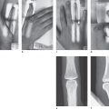
To acquire axial slices, the patient, wearing a lead apron, stands next to the CT gantry (Fig.8.2a). The patient’s forearm and hand are placed in pronation on a bocollo 10cm high so that the forearm-middle-finger axis is colinear and also the examined volume of the carpus is in the center of the gantry.
For examination of the scaphoid, the patient lies prone on the CT table and elevates the arm to be examined over his or her head. The pronated hand lying colinear to the forearm is positioned so that the forearm axis is at an angle of about 45° to the longitudinal dimension of the table (Fig.8.2b). The scaphoid and the slightly abducted thumb are then parallel to the scanning plane, which can be checked with the laser.
CT examination of the metacarpals and fingers is best performed in sagittal slices, which are parallel to the longitudinal axis of the phalanx (Fig.8.2c). Out-offield beam-hardening artifacts are best avoided by having the patient perform ulnar inclination of the wrist for examination of the index and middle fingers and radial inclination for examination of the ring and little fingers. This maneuver puts the forearm outside the scan plane.
For all positioning techniques, the hand and the forearm should be securely fixed to the CT table with wide adhesive strips. Positioning pads increase the patient’s comfort and help to avoid movement artifacts.
Planning Images
The localizers or “scouts” are acquired coronally in each case. A scout length of 15cm in the z direction is usually sufficient. After electronic magnification on the screen, the examined volume is defined by drawing in the starting line and the end of the scan, as well as by determining the scan FoV by means of two lateral lines. In CT of the scaphoid, it should be confirmed from the planning image that the scaphoid is aligned parallel to the scan plane (Fig.8.3). If necessary, the position should be corrected and the scout image repeated.
Acquisition Parameters and Dose
Typical acquisition parameters for CT examination of the wrist are a tube voltage of 120kV and a current-time product of 200–300 mAs. Depending on the CT scanner type, X-ray exposure is 15–30 mSv. Low-dose CT examinations with a voltage of 80kV and a current-time product of 100mAs are currently being tested for their diagnostic usefulness in the skeleton of the hand.
In examinations of the hand with a single-slice scanner, a slice thickness of 1mmwith a pitch factor of 1.3 and a reconstruction increment of 0.7 mm are recommended. For multislice spiral scanners, the following slice thicknesses are typical: 2×0.5mm, 4×0.5 mm, 8×0.5 mm, 16×0.5 mm, 64×0.4 mm, or 4×0.75 mm, 8×0.75 mm, 16×0.75 mm, and 64×0.5 mm. In this case, the pitch factor should also be set at about 1.3 and the reconstruction increment at 60–70% of the calculated slice thickness.

Depending on the constitution of the examined hand, for axial slices the field of view is set at a diameter of 60–80 mm. A larger FoV of the hand leads to a significant reduction in spatial resolution. For examination of the scaphoid, the oblique-sagittal slices should be limited to an FoV of 60 mm.

Intravenous administration of 100–150ml of a nonionic contrast medium is necessary only in the presence of inflammation or tumors or for CT angiography.
Image Computation
High-resolution image reconstruction is obligatory for CT imaging of the hand. Since CT is usually performed for assessment of the bony structures, image computation with an edge-enhancing algorithm (bone kernel) is important for the evaluation of axial source images (Fig.8.5) and the postprocessing of multiplanar reconstruction images (see below). For 3D surface-shaded reconstructions and volume-rendering, calculation of a second dataset with middle kernel significantly improves image quality.
The source planes acquired in the hand and the reconstructed planes, calculated afterwards, are compiled in Table 8.2.
Region Examined | Acquired Plane | Reformatted Planes (MPR) |
Distal section of forearm | Axial | Coronal and sagittal |
Entire carpus | Axial | Coronal and sagittal |
Scaphoid | Oblique-sagittal | Oblique-coronal |
Metacarpal region | Sagittal | Coronal (and axial if necessary) |
Finger | Sagittal | Coronal (and axial if necessary) |
Related posts:

Stay updated, free articles. Join our Telegram channel

Full access? Get Clinical Tree


