(1)
This makes sense heuristically because the more dense the material at x (i.e., the larger f(x) is), the more the beam is attenuated and the greater the decrease of I at x. Equation (1) is a simple differential equation for I that can be solved using separation of variables. If I 0 is the intensity at the X-ray emitter – the point x 0 ∈ ℓ – and I 1 is the intensity at the detector, x 1 ∈ ℓ, then one can integrate (1) to find
 was studied by the Austrian mathematician Johann Radon [84] in the early twentieth century because it was intriguing pure mathematics. This transform is called the Radon line transform (or X-ray transform).
To proceed mathematically, more notation is given. Let ω ∈ S 1 and let  . Then, the line
is perpendicular to ω and contains p ω. Sometimes it will be useful to let ω be a function of polar angle  ,
,
 In this parameterization
where  is the unit vector π∕2 radians counterclockwise from ω. This integral is defined for
  , and in fact
  is continuous in a number of norms (see section “Continuity Results for the X-Ray Transform”). The basic properties of this transform are proven in Sect. 3.
. Then, the line(2)
,(3)
is the unit vector π∕2 radians counterclockwise from ω. This integral is defined for , and in fact is continuous in a number of norms (see section “Continuity Results for the X-Ray Transform”). The basic properties of this transform are proven in Sect. 3.First, consider the forward problem and a simple case that will show in a naive sense how the X-ray transform detects object boundaries.
Example 1.
Let f be the characteristic function of the unit disk in  . Then, using the Pythagorean Theorem, one sees that
 in (4) is smooth except at p = ±1, that is, except for lines ℓ(ω, ±1) as can be seen from Fig. 1. The data are not smooth at those lines and those lines are tangent to the boundary of the disk. This suggests that lines tangent to boundaries give special information about the specimen. In Sect. 4, the reader will discover what is mathematically special about those lines, and this will be related back to limited data tomography in Sect. 5.
 is continuous.
Get Clinical Tree app for offline access

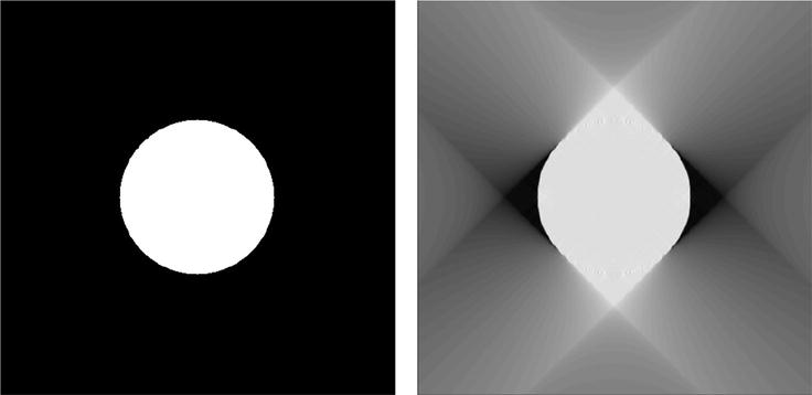
. Then, using the Pythagorean Theorem, one sees that in (4) is smooth except at p = ±1, that is, except for lines ℓ(ω, ±1) as can be seen from Fig. 1. The data are not smooth at those lines and those lines are tangent to the boundary of the disk. This suggests that lines tangent to boundaries give special information about the specimen. In Sect. 4, the reader will discover what is mathematically special about those lines, and this will be related back to limited data tomography in Sect. 5.Fig. 1
This graph shows the calculation of the Radon transform in (4). The unit disk is above the graph. For  , the Pythagorean theorem shows that the length of the intersection of ℓ(ω, p) and the disk is
, the Pythagorean theorem shows that the length of the intersection of ℓ(ω, p) and the disk is For complete data, that is, data over all lines through the object, good reconstruction methods such as filtered backprojection (Theorem 9) are effective to reconstruct from X-ray CT data.
However, one cannot obtain complete data in many important tomography problems. These are called limited data tomography problems, and several important ones are now described. The goal at this point is to observe how the reconstructions look compared to the original objects.
Here are some guidelines as you read this section. For each problem and reconstruction, conjecture what is special about the object boundaries that are well reconstructed (and those that are badly reconstructed) in relation to the limited data set used.
Exterior X-Ray CT Data
Exterior CT data are data for lines that are outside an excluded region. Typically, that region is a circle of radius r > 0, so lines ℓ(ω, p) for  are in the data set. Theorem 5 in the next section shows that compactly supported functions can be uniquely reconstructed outside the excluded region from exterior data.
are in the data set. Theorem 5 in the next section shows that compactly supported functions can be uniquely reconstructed outside the excluded region from exterior data.The exterior problem came about in the early days of tomography for CT scans around the beating heart. In those days, a single scan of a planar cross section could take several minutes, and movement of the heart would create artifacts in the scan. If an excluded region were chosen to contain the heart and be large enough so the outside of that region would not move, then data exterior to that region would be usable. However, scanners soon began to use fan beam data (see section “Fan Beam and Cone Beam CT”), and data could be acquired much more quickly. If the data acquisition is timed (gated), then data are acquired while the heart is in the same position over several heartbeats. Because more data can be taken more quickly with fan beam data, the heart can now be imaged using newer scanners, and movement of the heart is not as large a problem.
Exterior data are still important for imaging large objects such as rocket shells. Even with an industrial CT scanner, the X-rays will not penetrate the thick center of the rocket [88]. However, they can penetrate the outer rocket shell, and this gives exterior data.
One can recover functions of compact support from exterior data, at least outside the excluded region (see Theorem 5). Effective inversion methods were developed for exterior data by researchers including Bates and Lewitt [3], Natterer [65], Quinto [77, 79], and a stability analysis using singular value decompositions was done in [58].
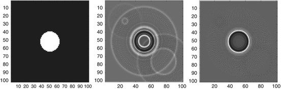
Figure 2 is a reconstruction from exterior data: integrals are given over lines that do not meet the black central disk.
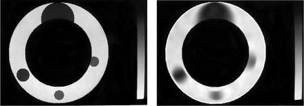
Fig. 2
Exterior reconstruction. Phantom (left) and reconstruction (right) from simulated data [77, ©IOP Publishing. Reproduced by permission of IOP Publishing. All rights reserved]. The outer diameter of the annulus is 1. 5 times the inner diameter
The reconstruction method uses a singular value decomposition for the exterior Radon transform that includes a null space; it recovers the component of the object in the orthogonal complement of the null space and does an extrapolation to recover the null space component [77].
Note how some boundaries of the small circles are clearly reconstructed and others are not. In this case, how can you describe the boundaries that are well reconstructed in relation to the data set? Another question is whether the fuzzy boundaries are fuzzy because the algorithm is bad or could there be an additional explanation.
Allan Cormack’s first algorithm [10] solved the exterior problem, but the algorithm was not numerically effective. The integrals in his algorithm were difficult to evaluate numerically with any accuracy because the integrand grew too rapidly. Other mathematicians tried to improve this method, but it was difficult. Because of this problem, Cormack developed a second method that uses full data and that gave good reconstructions [11].
It would be useful to know if limitations of Quinto’s and Cormack’s algorithms are problems with their algorithms or reflect something intrinsic to this limited data problem.
Limited Angle Data
Limited angle tomography is a classical problem from the early days of tomography [3, 60, 61]. In this case, data are given over all lines in a limited range of directions, or data for  where Φ ∈ (0, π∕2). One can uniquely recover compactly supported functions from limited angle data, but this is not true for arbitrary functions (see Theorem 3).
where Φ ∈ (0, π∕2). One can uniquely recover compactly supported functions from limited angle data, but this is not true for arbitrary functions (see Theorem 3).Limited angle tomography is used in certain luggage scanners in which the X-ray source is on one side of the luggage and the detectors are on the other, and they move in opposite directions. Limited angle data are used in important current problems including dental X-ray scanning [68] and tomosynthesis (a tomographic technique to image breasts using transmitter and receiver that move on opposite sides of the breast) [72]. Other algorithms were developed for this problem such as [12, 26, 49, 68].
The reconstruction in Fig. 3 is from limited angle data. Data are taken over all lines  for
for  and φ ∈ [−π∕4, π∕4].
for and φ ∈ [−π∕4, π∕4].Fig. 3
Limited angle reconstruction of a disk. Original image (left) and reconstruction (right) from a truncated filtered backprojection (FBP) algorithm (26) using data in the angular range, ![$$\varphi \in [-\pi /4,\pi /4]$$](/wp-content/uploads/2016/04/A183156_2_En_36_Chapter_IEq15.gif) . Note the streak artifacts and the missing boundaries in the limited angle reconstructions [26, ©IOP Publishing. Reproduced by permission of IOP Publishing. All rights reserved]
. Note the streak artifacts and the missing boundaries in the limited angle reconstructions [26, ©IOP Publishing. Reproduced by permission of IOP Publishing. All rights reserved]
. Note the streak artifacts and the missing boundaries in the limited angle reconstructions [26, ©IOP Publishing. Reproduced by permission of IOP Publishing. All rights reserved]The algorithm used in this reconstruction is a truncated filtered backprojection (FBP) algorithm which is given in (26). Some boundaries in this reconstruction are well reconstructed and others are not. How do these boundaries relate to lines in the data set? How do the streaks in the reconstruction relate to the data set?
Region of Interest (ROI) Data
In region of interest tomography, one chooses a subset of the object, called a region of interest (ROI), to reconstruct. ROI data consist of all lines that meet this region, and the ROI problem is to reconstruct the structure of the ROI from these data. Such data are also called interior data (and the interior problem). ROI CT is important in the CT of small parts of objects, so-called micro-CT [18, p. 460]. Other algorithms in ROI CT include [104] (when one knows the value of a function in part of the interior) and [105] (when the density is piecewise constant in the ROI), as well as algorithms including [52]. A singular value decomposition was developed for this problem in [63].
ROI CT is useful for medical CT and industrial nondestructive evaluation in which one is interested only in a small region of interest in an object, not the entire object. An advantage for medical applications is that ROI data gives less radiation than with complete data.
Lambda tomography [17], [18] is one important algorithm for ROI CT which will be described in section “Filtered Backprojection (FBP) for the X-Ray Transform,” and the ROI reconstruction presented here uses this algorithm. The data are severely limited – they include only lines near the disk and the ROI transform is not injective (see Theorem 6), so why do the reconstructions look so good?
Limited Angle Region of Interest Tomography
In this modality data are given over lines in a limited angular range and that are restricted to pass through a given ROI. It comes up in single axis tilt electron microscopy (ET) (see Öktem’s chapter in this book [71]). However, in general, ET is better understood as a three-dimensional problem, and this will be presented in the next paragraph.
Electron Microscope Tomography (ET) Over Arbitrary Curves
Now a full three-dimensional problem, electron microscope tomography (ET), is considered. The notation is as in Öktem’s chapter in this book [71], which has detailed information about the physics, biology, model, and mathematics of ET. A reconstruction of a simple 3D phantom – the union of the following disks: with center (0, 0, 0), radius 1∕2; center (0, 0, 1), radius 1∕2; center (1, −1, 1), radius 1∕4; and center (−1, 1, −1∕2), radius 1∕4 – is analyzed. The disks above the x − y plane have density two and the others have density one.
Conical tilt ET data is described in section “Algorithms in Conical Tilt ET” and Öktem’s chapter in this book [71]. In this example, line integrals are given over all lines in space with angle α = π∕4 with the z−axis. Reconstructions are given from two algorithms that are described in section “Electron Microscope Tomography (ET) Over Arbitrary Curves.” The operators are  (given in Eq. (28)) and
  (given in Eq. (29)).
(given in Eq. (28)) and (given in Eq. (29)).Artifacts are added in the  reconstruction in Fig. 4 and in Fig. 5 which shows the plane containing the centers of the disks and the z−axis (axis of rotation of the scanner).
reconstruction in Fig. 4 and in Fig. 5 which shows the plane containing the centers of the disks and the z−axis (axis of rotation of the scanner).Fig. 4
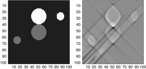
Reconstruction from conical tilt data. Cross section with the x − y plane of the phantom described in this section (left),  reconstruction (center, see Eq. (28)) and
  reconstruction (right, see Eq. (29)). The center of the cross section is the origin, and the range in x and y is from − 2 to 2. This research was done with Sohhyun Chung and Tania Bakhos while they were Tufts undergraduates [82, ©Scuola Normale Superiore, Pisa. Reproduced by permission with Scuola Normale Superiore, Pisa, all rights reserved]
reconstruction (center, see Eq. (28)) and reconstruction (right, see Eq. (29)). The center of the cross section is the origin, and the range in x and y is from − 2 to 2. This research was done with Sohhyun Chung and Tania Bakhos while they were Tufts undergraduates [82, ©Scuola Normale Superiore, Pisa. Reproduced by permission with Scuola Normale Superiore, Pisa, all rights reserved]Fig. 5
Reconstruction from conical tilt data. Cross section of phantom in the plane x = −y (left) and  reconstruction in that plane (right). The x − y plane cuts the picture in half with a horizontal line [82, ©Scuola Normale Superiore, Pisa. Reproduced by permission with Scuola Normale Superiore, Pisa, all rights reserved]
reconstruction in that plane (right). The x − y plane cuts the picture in half with a horizontal line [82, ©Scuola Normale Superiore, Pisa. Reproduced by permission with Scuola Normale Superiore, Pisa, all rights reserved]These figures are remarkable because the  reconstruction has so many added artifacts compared to the
  reconstruction, although these operators are not very different (see section “Algorithms in Conical Tilt ET”). Why are the reconstructions so different?
reconstruction has so many added artifacts compared to the reconstruction, although these operators are not very different (see section “Algorithms in Conical Tilt ET”). Why are the reconstructions so different?Synthetic-Aperture Radar Imaging
In synthetic-aperture radar (SAR) imaging, a region of interest on the surface of the earth is illuminated by electromagnetic waves from an airborne platform such as a plane or satellite. For more detailed information on SAR imaging, including several open problems in SAR imaging, the reader is referred to [7, 8] and to the chapter in this handbook by Cheney and Borden [9]. The backscattered waves are picked up at a receiver or receivers, and the goal is to reconstruct an image of the region based on such measurements. In monostatic SAR, the transmitter and receiver are located on the same platform. In bistatic SAR, the transmitter and receiver are on independently moving trajectories.
While monostatic SAR imaging is the one that is widely used, bistatic SAR imaging offers several advantages. The receivers in comparison to transmitters are not active sources of electromagnetic radiation and hence are more difficult to detect if flown in an unsafe environment. Since the transmitter and receiver are at different points in space, bistatic SAR systems are more resistant to electronic countermeasures such as target shaping to reduce scattering in the direction of incident waves [48].
The reconstruction of the image based on the measurement of the backscattered waves is in general a hard problem. However, ignoring contributions of multiply backscattered waves linearizes the relation between the image to be recovered and the backscattered waves and is easier to analyze. Due to this reason, a linearizing approximation called the Born approximation that ignores contribution from multiply scattered waves is widely used in SAR image reconstruction.
The Linearized Model in SAR Imaging
Let γ T (s) and γ R (s) for s ∈ (s 0, s 1) be the trajectories of the transmitter and receiver, respectively. The propagation of electromagnetic waves can be described by the scalar wave equation
where c is the speed of electromagnetic waves in the medium, E(x, t) is each component of the electric field, and P(t) is the transmit waveform sent to the transmitter antenna. The wave speed c is spatially varying due to inhomogeneities present in the medium, and one can assume that it is a perturbation of the constant background speed of propagation c 0 of the form
 One assumes that
  only varies over a two-dimensional surface: the surface of the earth. Therefore,
  can be represented as a function of the form
 where it will be assumed that the earth’s surface is represented by the x = (x 1, x 2) plane. The background Green’s function g is the solution of the following equation:
 This is given by
Now the incident field E in due to the source s(x, t) = P(t)δ(x −γ T (s)) is
 Let E denote the total field of the medium, E = E in + E sc, where E sc is the scattered field. This can be written using the Lippmann-Schwinger equation:
This equation is linearized by replacing the total field E on the right-hand side of the above equation by E in. This is known as the Born approximation. The linearized scattered wave field E lin sc(γ R (s), t) at the receiver location γ R (s) is then
 Substituting the expression for E in into this equation and integrating, one obtains the following expression for the linearized scattered wave field:
where
 and
and

where p is the Fourier transform of P. The function A includes terms that take into account the transmitted waveform and geometric spreading factors. The inverse of the norms appears in A due to the background Green’s function, (6).
(5)
only varies over a two-dimensional surface: the surface of the earth. Therefore, can be represented as a function of the form(6)
(7)
(8)
(9)
The reconstruction in Fig. 6 of a disk centered on the positive y-axis from integrals of it over ellipses with foci moving along the x-axis offset by a constant distance (which is simplified model of (8)) highlights some of the features in SAR image reconstruction. Some part of the boundary is not stably reconstructed, and an artifact of the true image appears as a reflection about the x-axis along with streak artifacts. Looking at the reconstructed image, one sees that at least visually, the created artifact is as strong as the true image. Microlocal analysis of the operators appearing in SAR imaging will make precise and justify all these observations. This will be addressed in section “SAR Imaging.”
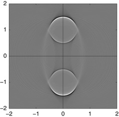
Fig. 6
Reconstruction of a disk centered on the positive y-axis from integrals over ellipses (with constant distance between the foci) centered on the x-axis and with foci in [−3,3]. Notice that some boundaries of the disk are missing, and there is a copy of the disk below the axis. This was originally from the Tufts University Senior Honors thesis of Howard Levinson and published in [55, Reproduced with kind permission from Springer Science+Business Media: © Springer Verlag]
General Observations
In each reconstruction in this section, some object boundaries are visible and others are not. In fact, if one looks more carefully at the reconstructions, one can notice that in each case, the only feature boundaries that are clearly defined are those tangent to lines in the data set for the problem. Example 1 illustrates this in a naive way: one sees singularities in the Radon data exactly when the lines of integration are tangent to the boundary of the object. The goal of this chapter is to make the idea mathematically rigorous.
The conical tilt ET reconstructions in section “Electron Microscope Tomography (ET) Over Arbitrary Curves” have artifacts if one uses a certain algorithm but apparently not when one uses another similar one. The reconstruction related to radar in Fig. 6 has an artifact that is a reflected image of the disk.
In Sect. 4, deep mathematical ideas from microlocal analysis will be introduced to classify singularities and what certain operators do to them. In Sect. 5 these microlocal ideas will be used to explain the visible and invisible singularities for limited data X-ray CT as well as the added singularities in ET and radar.
3 Properties of Tomographic Transforms
In this section, after introducing some functional analysis, basic properties of transforms in X-ray tomography and electron microscope tomography are presented. The microlocal properties of radar will be given later in section “SAR Imaging.”
Function Spaces
The open disk in  centered at the origin and of radius r > 0 will be denoted D(r).
centered at the origin and of radius r > 0 will be denoted D(r).The set  consists of all smooth functions on
  , that is, functions that are continuous along with their derivatives of all orders, and
  is the set of smooth functions of compact support. Its dual space – the set of all continuous linear functionals on
  (given the weak-* topology) – is denoted
  and is called the set of distributions. If u is a locally integrable function, then u is a distribution with the standard definition
 for
for  since u(x)f(x) is an integrable function of compact support.
consists of all smooth functions on , that is, functions that are continuous along with their derivatives of all orders, and is the set of smooth functions of compact support. Its dual space – the set of all continuous linear functionals on (given the weak-* topology) – is denoted and is called the set of distributions. If u is a locally integrable function, then u is a distribution with the standard definition since u(x)f(x) is an integrable function of compact support.If Ω is an open set in  , then
  is the set of smooth functions compactly supported in Ω. Its dual space with the weak-* topology is denoted
  .
.
, then is the set of smooth functions compactly supported in Ω. Its dual space with the weak-* topology is denoted .The Schwartz space of rapidly decreasing functions is the set  of all smooth functions that decrease (along with all their derivatives) faster than any power of
  at infinity. Its dual space,
  , is the set of all continuous linear functionals on
  with the weak-* topology (convergence is pointwise: u k → u in
  if, for each
  , u k (f) → u(f)). They are called tempered distributions. Any function that is measurable and bounded above by some power of
  is in
is in  since its product with any Schwartz function is integrable.
of all smooth functions that decrease (along with all their derivatives) faster than any power of at infinity. Its dual space, , is the set of all continuous linear functionals on with the weak-* topology (convergence is pointwise: u k → u in if, for each , u k (f) → u(f)). They are called tempered distributions. Any function that is measurable and bounded above by some power of is in since its product with any Schwartz function is integrable.A distribution u is supported in the closed set K if for all functions  with support disjoint from K, u(f) = 0. The support of u,
  , is the smallest closed set in which u is supported.
with support disjoint from K, u(f) = 0. The support of u, , is the smallest closed set in which u is supported.Example 2.
The Dirac delta function at zero is an important distribution that is not a function. It is defined  . Note that if f is supported away from the origin, then δ 0(f) = 0 since f(0) = 0. Therefore, the Dirac delta function has support
  .
.
. Note that if f is supported away from the origin, then δ 0(f) = 0 since f(0) = 0. Therefore, the Dirac delta function has support .Let  be the set of distributions that have compact support in
  . If Ω is an open set in
  , then
  is the set of distributions with compact support contained in Ω. For example, on the real line,
  .
.
be the set of distributions that have compact support in . If Ω is an open set in , then is the set of distributions with compact support contained in Ω. For example, on the real line, .If  , then its Fourier transform and inverse are
The Fourier transform is linear and continuous from  to the space of continuous functions that converge to zero at ∞. Furthermore,
  is an isomorphism on
  and an isomorphism on
  and, therefore, on
  . More information about these topics can be found in [86], for example.
, then its Fourier transform and inverse are(10)
to the space of continuous functions that converge to zero at ∞. Furthermore, is an isomorphism on and an isomorphism on and, therefore, on . More information about these topics can be found in [86], for example. Basic Properties of the Radon Line Transform
In this section fundamental properties of the Radon line transform,  , are derived, see [66]. This will provide a connection between the transforms and microlocal analysis in Sect. 4.
, are derived, see [66]. This will provide a connection between the transforms and microlocal analysis in Sect. 4.Theorem 1 (General Projection Slice Theorem).
Let  . Now let
  and ω ∈ S 1. Then,
. Now let and ω ∈ S 1. Then,(11)
Proof.


Let  be the set of smooth functions on
  that decrease (along with all their derivatives) faster than any power of
  at infinity uniformly in ω, and let
  be its dual. The partial Fourier transform is defined for
  as
as
Because the Fourier transform is an isomorphism on  , this transform and its inverse are defined and continuous on
  .
.
be the set of smooth functions on that decrease (along with all their derivatives) faster than any power of at infinity uniformly in ω, and let be its dual. The partial Fourier transform is defined for as(14)
, this transform and its inverse are defined and continuous on .The Fourier Slice Theorem is an important corollary of Theorem 1.
Theorem 2 (Fourier Slice Theorem).
Let  . Then for
  ,
,
. Then for ,To prove this theorem, one applies the General Projection Slice Theorem 1 to the function  .
.
.The Fourier Slice Theorem provides a proof that  is invertible on domain
  since
since  is invertible on domain
  . Zalcman constructed a nonzero function that is integrable on every line in the plane and whose line transform is identically zero [107]. Of course, his function is not in
  .
.
is invertible on domain since is invertible on domain . Zalcman constructed a nonzero function that is integrable on every line in the plane and whose line transform is identically zero [107]. Of course, his function is not in .This theorem also provides a proof of invertibility for the limited angle problem.
Theorem 3 (Limited Angle Theorem).
Let  and let Φ ∈ (0,π∕2). If
  for
for  and all p, then f = 0.
and let Φ ∈ (0,π∕2). If for and all p, then f = 0. However, there are nonzero functions  with
with  for φ ∈ (−Φ,Φ) and all p.
with for φ ∈ (−Φ,Φ) and all p. Proof.
Let  and assume
  for φ ∈ (−Φ, Φ) and all p. By the Fourier Slice Theorem, which is true for
  [45],
[45],
and this expression is zero because  for such (φ, τ). This shows that
  is zero on the open cone
 Since f has compact support,
  is real analytic, and so
  must be zero everywhere since it is zero on the open set V. This shows f = 0.
and assume for φ ∈ (−Φ, Φ) and all p. By the Fourier Slice Theorem, which is true for [45],(15)
for such (φ, τ). This shows that is zero on the open cone is real analytic, and so must be zero everywhere since it is zero on the open set V. This shows f = 0.To prove the second part of the theorem, let  be any nonzero Schwartz function supported in the cone V and let
  . Since
  is nonzero and in
  , so is f. Using (15) but starting with
  in V, one sees that
  is zero in the limited angular range. □
be any nonzero Schwartz function supported in the cone V and let . Since is nonzero and in , so is f. Using (15) but starting with in V, one sees that is zero in the limited angular range. □Another application of these theorems is the classical Range Theorem for this transform.
Let  . Then g is in the range of
  on domain
  if and only if
. Then g is in the range of on domain if and only if 1.
 for all
for all 2.
For each  ,
,  is a polynomial in ω ∈ S1 that is homogeneous of degree m.
, is a polynomial in ω ∈ S1 that is homogeneous of degree m.Proof (Sketch).
The necessary part of the theorem follows by applying the General Projection Slice Theorem to h(p) = p m for m a nonnegative integer:
 and after multiplying out
  in the coordinates of ω, one sees that the right-hand integral is a polynomial in these coordinates homogeneous of degree m. The sufficiency part is much more difficult to prove. One uses the Fourier Slice Theorem to construct a function f satisfying
  . Since
  is smooth and rapidly decreasing in p,
  is smooth away from the origin and rapidly decreasing in x. The subtle part of the proof in [41] is to show
  is smooth at the origin, and this is done using careful estimates on derivatives using the moment conditions, (2) of Theorem 4. Once that is known, one can conclude
  and so
  . □
. □
in the coordinates of ω, one sees that the right-hand integral is a polynomial in these coordinates homogeneous of degree m. The sufficiency part is much more difficult to prove. One uses the Fourier Slice Theorem to construct a function f satisfying . Since is smooth and rapidly decreasing in p, is smooth away from the origin and rapidly decreasing in x. The subtle part of the proof in [41] is to show is smooth at the origin, and this is done using careful estimates on derivatives using the moment conditions, (2) of Theorem 4. Once that is known, one can conclude and so . □The support theorem for  is elegant and has motivated a large range of generalizations such as [5, 6, 42, 53, 57, 78].
is elegant and has motivated a large range of generalizations such as [5, 6, 42, 53, 57, 78].Let f be a distribution of compact support (or a function in  ) and let r > 0. Assume
  is zero for all lines that are disjoint from the disk D(r). Then
  .
.
) and let r > 0. Assume is zero for all lines that are disjoint from the disk D(r). Then .This theorem implies that the exterior problem has a unique solution; in this case, D(r) is the excluded region. The proof is tangential to the main topics of this chapter, and it can be found in [10, 28, 41, 43, 92].
Counterexamples to the support theorem exist for functions that do not decrease rapidly at ∞ (e.g., [43, 106] or the singular value decompositions in [73, 76]).
A corollary of these theorems shows that exact reconstruction is impossible from ROI data where D(r) is the disk centered at the origin in  and of radius r > 0.
and of radius r > 0.Theorem 6.
Consider the ROI problem with region of interest the unit disk D(1). Let r ∈ (1,∞). Then there is a function  that is not identically zero in D(1) but for which
  is zero for all lines that intersect D(1).
that is not identically zero in D(1) but for which is zero for all lines that intersect D(1). Proof (Sketch).
Let h(p) be a smooth nonzero nonnegative function supported in (1, r) and let  . Since g is independent of ω, the moment conditions from the Range Theorem (Theorem 4), are trivially satisfied, so that theorem shows that there is a function
  with
with  . By the support theorem, f is supported in the disk D(r). To show f is nonzero in the ROI, D(1), one uses [10, p. 2725, equation (18)]. This is also proven in [66, p. 169, VI.4], and Natterer shows that such null functions do not oscillate much in the ROI. It will be shown in Sect. 5 that null functions are smooth in the ROI, too. □
. Since g is independent of ω, the moment conditions from the Range Theorem (Theorem 4), are trivially satisfied, so that theorem shows that there is a function with . By the support theorem, f is supported in the disk D(r). To show f is nonzero in the ROI, D(1), one uses [10, p. 2725, equation (18)]. This is also proven in [66, p. 169, VI.4], and Natterer shows that such null functions do not oscillate much in the ROI. It will be shown in Sect. 5 that null functions are smooth in the ROI, too. □Continuity Results for the X-Ray Transform
In this section some basic continuity theorems for  are presented.
are presented.A simple proof shows that  is continuous from C c (D(M)) to C c (S M ) where we define S M = S 1 × [−M, M]. First, one uses uniform continuity of f to show
  is a continuous function. Then, the proof that
  is continuous is based on the estimate
 where
where  is the (essential) supremum norm of f. A stronger theorem has been proven by Helgason.
is continuous from C c (D(M)) to C c (S M ) where we define S M = S 1 × [−M, M]. First, one uses uniform continuity of f to show is a continuous function. Then, the proof that is continuous is based on the estimate is the (essential) supremum norm of f. A stronger theorem has been proven by Helgason.
The proof of the next theorem follows from the calculations in the proof of the General Projection Slice Theorem.
Theorem 8.
is continuous. Proof.
By taking absolute values in (11) with h = 1 and then integrating with respect to ω, one sees that  and so
  is continuous on L 1. □
and so is continuous on L 1. □
Filtered Backprojection (FBP) for the X-Ray Transform
To state the most commonly used inversion formula, filtered backprojection, one first defines the dual line transform. For  and
and  ,
,
For each ω ∈ S 1, x ∈ ℓ(ω, x ⋅ ω), so  is the integral of g over all lines through x. The transform
  is the formal dual to
  in the sense that for
  and
and  ,
,
 Because
  is continuous,
  is weakly continuous.
and ,(16)
is the integral of g over all lines through x. The transform is the formal dual to in the sense that for and , is continuous, is weakly continuous.The Lambda operator is defined on functions  by
by
by(17)


Filtered backprojection is an efficient, fast reconstruction method that is easily implemented [67] by using an approximation to the operator Λ p that is convolution with a function (see, e.g., [66] or [87]). Note that FBP requires data over all lines through the object – it is not local: in order to find f(x), one needs data  over all lines in order to evaluate
  (which involves a Fourier transform).
over all lines in order to evaluate (which involves a Fourier transform).To see the how sensitive FBP is to the number of the angles used, reconstructions are provided in Fig. 7 using 18, 36, and 180 angles. One can see that using too few angles creates artifacts. An optimal choice of angles and values of p can be determined using sampling theory [15, 16, 66].
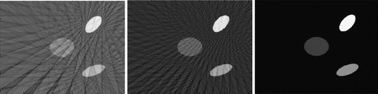
Fig. 7
FBP reconstructions of phantom consisting of three ellipses. The left reconstruction uses 18 angles, the middle 36 angles, and the right one 180 angles
Proof (Proof of Theorem 9).
Let  . First, one writes the two-dimensional Fourier inversion formula in polar coordinates:
The factor of 1∕2 in front of the integral in (19) occurs because the integral is over  rather than τ ∈ [0, ∞). The Fourier Slice Theorem (Theorem 2) is used in (20), and the definitions of Λ p and of
  are used in (21). The integrals above exist because f,
  , and
, and  are all rapidly decreasing at infinity.
. First, one writes the two-dimensional Fourier inversion formula in polar coordinates:(19)
(20)
(21)
rather than τ ∈ [0, ∞). The Fourier Slice Theorem (Theorem 2) is used in (20), and the definitions of Λ p and of are used in (21). The integrals above exist because f, , and are all rapidly decreasing at infinity.The proof that the FBP formula is valid for  will now be given. Since
  , the Fourier Slice Theorem holds for f [45], and
 is a smooth function that is polynomially increasing [86]. So,
  is a polynomially increasing continuous function and therefore in
  . Since the inverse Fourier transform,
  , maps
  to
to  ,
,  is a distribution in
  . By duality with
  ,
,  , so
, so  is defined for
  . Since the Fourier Slice Theorem holds for f [45], the FBP formula can be proved for f as is done above for
  (see [26] more generally). □
will now be given. Since , the Fourier Slice Theorem holds for f [45], and is a polynomially increasing continuous function and therefore in . Since the inverse Fourier transform, , maps to , is a distribution in . By duality with , , so is defined for . Since the Fourier Slice Theorem holds for f [45], the FBP formula can be proved for f as is done above for (see [26] more generally). □Limited Data Algorithms
In limited data problems, some data are missing, and reconstruction methods are now presented for ROI CT, limited angle CT, and limited angle ROI CT.
ROI Tomography
Lambda tomography [17, 18, 96] is an effective and easy-to-implement algorithm for ROI CT. The fundamental idea is to replace Λ p by − d 2∕dp 2 in the FBP formula. The relation between these two operators is that Λ p 2 = −d 2∕dp 2, which will be justified in Example 9. This motivates the definition
(22)
FBP is not local; to calculate  , one needs data over all lines to take the Fourier transform
  . Therefore, one needs data over all lines through the object to calculate f using FBP (18). This means that FBP cannot be used on ROI data.
, one needs data over all lines to take the Fourier transform . Therefore, one needs data over all lines through the object to calculate f using FBP (18). This means that FBP cannot be used on ROI data.The advantage of Lambda tomography over FBP is that  is local in the following sense. To calculate
  , one needs the values of
  at all lines through x (since
  evaluated at x integrates over all such lines). Furthermore,
  is a local operator, and to calculate
  at a line through x, one needs only data
  over lines close to x. Therefore, one needs only data over all lines near x to calculate
  . Therefore,
  can be used on ROI data. Although Lambda CT reconstructs
  , not f itself, it shows boundaries very clearly (see Fig. 8 and [17]).
is local in the following sense. To calculate , one needs the values of at all lines through x (since evaluated at x integrates over all such lines). Furthermore, is a local operator, and to calculate at a line through x, one needs only data over lines close to x. Therefore, one needs only data over all lines near x to calculate . Therefore, can be used on ROI data. Although Lambda CT reconstructs , not f itself, it shows boundaries very clearly (see Fig. 8 and [17]).

Kennan Smith developed an improved local operator that shows contours of objects, not just boundaries. His idea was to add a positive multiple of  to the reconstruction to get
for some μ > 0. Using (35), one sees that
so this factor adds contour to the reconstruction since the convolution with  emphasizes the values of f near x. Lambda reconstructions look much like FBP reconstructions even though they are local. A discussion of how to choose μ to counteract a natural cupping effect of
  is given in [17]. The operator
  is local for the same reasons as
  is, and it was used in the ROI reconstruction in Fig. 8.
to the reconstruction to get(23)
(24)
emphasizes the values of f near x. Lambda reconstructions look much like FBP reconstructions even though they are local. A discussion of how to choose μ to counteract a natural cupping effect of is given in [17]. The operator is local for the same reasons as is, and it was used in the ROI reconstruction in Fig. 8.Limited Angle CT
There are several algorithms for limited angle tomography (e.g., [3, 12, 49, 61, 104]), and two will be presented that are generalizations of FBP and Lambda CT. The key to each is to use the limited angle backprojection operator that uses angles in an interval (−Φ, Φ) with Φ ∈ (0, π∕2):
The limited angle FBP and limited angle Lambda algorithms are
respectively. The objects in Fig. 3 are reconstructed using this limited angle FBP algorithm. Limited angle Lambda CT is local, so it can be used for the limited angle ROI data in electron microscope tomography [80, 83].
(25)
(26)
Fan Beam and Cone Beam CT
The parallel beam parameterization of lines in the plane used above is more convenient mathematically, but modern CT scanners use a single X-ray source that emits X-rays in a fan or cone beam. The source and detectors (on the other side of the body) move around the body and quickly acquire data. This requires different parameterizations of lines.
The fan beam parameterization is used if the X-rays are collimated to one reconstruction plane. Let C be the curve of sources in the plane, typically a circle surrounding the object, and let (ω, θ) ∈ C × S 1. Then,
 In this case the analogs of the formulas proved above are a little more complicated. For example, a Lambda-type operator can be designed by taking the negative second derivative in θ ∈ S 1. The other formulas are similar and one can find them in [66, 90].
In cone beam tomography, the source is collimated to illuminate a cone in space, and the source moves in a curve around the body along with the detectors. This scanner images a volume in the body, rather than a planar region as  , and the fan beam transform does. However, the reconstruction formulas are more subtle [50], and one can understand these difficulties using microlocal analysis [25, 30]. Related issues come up in conical tilt ET as will be described in section “Microlocal Analysis of Conical Tilt Electron Microscope Tomography (ET).”
, and the fan beam transform does. However, the reconstruction formulas are more subtle [50], and one can understand these difficulties using microlocal analysis [25, 30]. Related issues come up in conical tilt ET as will be described in section “Microlocal Analysis of Conical Tilt Electron Microscope Tomography (ET).”These data acquisition methods have several advantages over parallel beam data acquisition. First, the scanners are simpler to build than the original CT scanners, which took data using the parallel geometry, and so a single X-ray source (or several collimated sources) and detector(s) were translated to get data over parallel lines in one direction, and then the source and detector were rotated to get lines for other directions. Second, they can acquire data more quickly than old style parallel beam scanners since the fan beam X-ray source and detector array move in a circle around the object.
This is all discussed in Herman’s chapter in this book [44].
Algorithms in Conical Tilt ET
Conical tilt ET [108] is a new data acquisition geometry in ET that has the potential to provide faster data acquisition as well as clearer reconstructions. The algorithms used for the conical tilt ET reconstructions will be given in section “Electron Microscope Tomography (ET) Over Arbitrary Curves.” This will lay the groundwork to understand why the reconstructions in that section from two very similar algorithms are so dramatically different. The model and mathematics are fully discussed in Öktem’s chapter in this book [71].
First the notation is established. For ω ∈ S 2, denote the plane through the origin perpendicular to ω by
The tangent space to the sphere S 2 is
 since the plane ω P is the tangent plane to S 2 at ω. This gives the parallel beam parameterization of lines in space: for (ω, x) ∈ T(S 2), the line
 If ω is fixed, then the lines L(ω, x) for x ∈ ω P are all parallel. As noted in Öktem’s chapter in this book [71], ET data are typically taken on a curve S ⊂ S 2. This means the lines in the data set are parameterized by
 So, for
  , the ET data of f for lines parallel to S can be modeled as the parallel beam transform
 Its dual transform is defined for functions g on
  as
as
 where dω is the arc length measure on S. This represents the integral of g over all lines through x.
(27)
, the ET data of f for lines parallel to S can be modeled as the parallel beam transform asIn this section, conical tilt ET is considered; an angle α ∈ (0, π∕2) is chosen, and data are taken for angles on the latitude circle:
![$$\displaystyle{S_{\alpha } =\{ \left (\sin (\alpha )\cos (\varphi ),\sin (\alpha )\sin (\varphi ),\cos (\alpha )\right )\}\,:\,\varphi \in [0,2\pi ]\}.}$$](/wp-content/uploads/2016/04/A183156_2_En_36_Chapter_Equw.gif) Let C α be the cone with vertex at the origin and opening angle α from the vertical axis:
Let C α be the cone with vertex at the origin and opening angle α from the vertical axis:
 Note that C α is the cone generated by S α .
Here are the two algorithms for which reconstructions were given in section “Electron Microscope Tomography (ET) Over Arbitrary Curves.” The first operator is a generalization of one developed for cone beam CT by Louis and Maaß [62]:
where Δ S is the Laplacian on the detector plane, ω P . The second operator is defined
where  is the second derivative on the detector plane ω P in the tangent direction to the curve S at ω (see Öktem’s chapter in this book [71]). The next theorem helps clarify these operators by writing them as convolution operators.
(28)
(29)
is the second derivative on the detector plane ω P in the tangent direction to the curve S at ω (see Öktem’s chapter in this book [71]). The next theorem helps clarify these operators by writing them as convolution operators.Theorem 10.
Let  be the conical tilt ET transform with angle α ∈ (0,π∕2). Let
  . Then
where I is the distribution defined for  by
by
 and d y is the surface area measure on the cone C α.
be the conical tilt ET transform with angle α ∈ (0,π∕2). Let . Then(30)
(31)
(32)
byEquation (30) makes sense since  integrates
  over all lines in the data set through x, and these are exactly the lines in the shifted cone x + C α . The theorem implies that each of the operators is related to a simple convolution with a singular weighted integration over the cone C α .
integrates over all lines in the data set through x, and these are exactly the lines in the shifted cone x + C α . The theorem implies that each of the operators is related to a simple convolution with a singular weighted integration over the cone C α .Proof.
The theorem is first proven for  , by calculating (30):
 where the substitution s = t − (x
 Segmentation with Shape Priors: Explicit Versus Implicit Representations
 Transform in Astronomical Data Processing
 Methods for Multi-dimensional Visual Data Analysis
 Set Methods for Structural Inversion and Image Reconstruction
 Methods for Ill-Posed Problems
 and Shah Model and Its Applications to Image Segmentation and Image Restoration


, by calculating (30):Related posts:
Segmentation with Shape Priors: Explicit Versus Implicit Representations
Set Methods for Structural Inversion and Image Reconstruction
Stay updated, free articles. Join our Telegram channel
Full access? Get Clinical Tree