Fig. 1
Example of astronomical data: a point source and an extended source are shown, with noise and background. The extended object, which can be detected by eye, is undetected by a standard detection approach
2 Standard Approaches to Source Detection
We describe here the most popular way to create a catalog of galaxies from astronomical images.
The Traditional Data Model
The observed data Y can be decomposed into two parts, the signal X and the noise N:
![$$\displaystyle{ Y [k,l] = X[k,l] + N[k,l] }$$](/wp-content/uploads/2016/04/A183156_2_En_34_Chapter_Equ1.gif)
The imaging system can also be considered. If it is linear, the relation between the data and the image in the same coordinate frame is a convolution:
![$$\displaystyle\begin{array}{rcl} Y [k,l]& =& (HX)[k,l] + N[k,l]{}\end{array}$$](/wp-content/uploads/2016/04/A183156_2_En_34_Chapter_Equ2.gif)
where H is the matrix related to the point spread function (PSF) of the imaging system.
(1)
(2)
In most cases, objects of interest are superimposed on a relatively flat signal B, called background signal. The model becomes
![$$\displaystyle{ Y [k,l] = (HX)[k,l] + B[k,l] + N[k,l] }$$](/wp-content/uploads/2016/04/A183156_2_En_34_Chapter_Equ3.gif)
(3)
PSF Estimation
The PSF H can be estimated from the data or from an optical model of the imaging telescope. In astronomical images, the data may contain stars, or one can point towards a reference star in order to reconstruct a PSF. The drawback is the “degradation” of this PSF because of unavoidable noise or spurious instrument signatures in the data. So, when reconstructing a PSF from experimental data, one has to reduce very carefully the images used (background removal for instance). Another problem arises when the PSF is highly variable with time, as is the case for adaptive optics (AO) images. This means usually that the PSF estimated when observing a reference star, after or before the observation of the scientific target, has small differences from the perfectly correct PSF.
Another approach consists of constructing a synthetic PSF. Various studies [11, 21, 38, 39] have suggested a radially symmetric approximation to the PSF:
The parameters β and R are obtained by fitting the model with stars contained in the data.
(4)
In the case of AO systems, this model can be used for the tail of the PSF (the so-called seeing contribution), while in the central region, the system provides an approximation of the diffraction-limited PSF. The quality of the approximation is measured by the Strehl ratio (SR), which is defined as the ratio of the observed peak intensity in the image of a point source to the theoretical peak intensity of a perfect imaging system.
Background Estimation
The background must be accurately estimated; otherwise it will introduce bias in flux estimation. In [7, 28], the image is partitioned into blocks, and the local sky level in each block is estimated from its histogram. The pixel intensity histogram p(Y ) is modeled using three parameters, the true sky level B, the RMS (root mean square) noise σ, and a parameter describing the asymmetry in p(Y ) due to the presence of objects, and is defined by [7]:
![$$\displaystyle{ p(Y ) = \frac{1} {a}\exp \left (\sigma ^{2}/2a^{2}\right )\exp \left [-(Y - B)/a\right ]{\mathrm{erfc}}\left ( \frac{\sigma } {a} -\frac{(Y - B)} {\sigma } \right ) }$$](/wp-content/uploads/2016/04/A183156_2_En_34_Chapter_Equ5.gif)
(5)
Median filtering can be applied to the 2D array of background measurements in order to correct for spurious background values. Finally the background map is obtained by a bilinear or a cubic interpolation of the 2D array. The block size is a crucial parameter. If it is too small, the background estimation map will be affected by the presence of objects, and if too large it will not take into account real background variations.
In [6, 15], the local sky level is calculated differently. A 3-sigma clipping around the median is performed in each block. If the standard deviation is changed by less than 20 % in the clipping iterations, the block is uncrowded, and the background level is considered to be equal to the mean of the clipped histogram. Otherwise, it is calculated by c 1 ×median − c 2 ×mean, where  in [15] and
  in [6]. This approach has been preferred to histogram fitting for two reasons: it is more efficient from the computation point of view and more robust with small sample size.
in [15] and in [6]. This approach has been preferred to histogram fitting for two reasons: it is more efficient from the computation point of view and more robust with small sample size.Convolution
In order to optimize the detection, the image must be convolved with a filter. The shape of this filter optimizes the detection of objects with the same shape. Therefore, for star detection, the optimal filter is the PSF. For extended objects, a larger filter size is recommended. In order to have optimal detection for any object size, the detection must be repeated several times with different filter sizes, leading to a kind of multiscale approach.
Detection
Once the image is convolved, all pixels Y [k, l] at location (k, l) with a value larger than T [k, l] are considered as significant, i.e., belonging to an object. T [k, l] is generally chosen as B [k, l] + K σ, where B [k, l] is the background estimate at the same position, σ is the noise standard deviation, and K is a given constant (typically chosen between 3 and 5). The thresholded image is then segmented, i.e., a label is assigned to each group of connected pixels. The next step is to separate the blended objects which are connected and have the same label.
An alternative to the thresholding/segmentation procedure is to find peaks. This is only well suited to star detection and not to extended objects. In this case, the next step is to merge the pixels belonging to the same object.
Deblending/Merging
This is the most delicate step. Extended objects must be considered as single objects, while multiple objects must be well separated. In SExtractor, each group of connected pixels is analyzed at different intensity levels, starting from the highest down to the lowest level. The pixel group can be seen as a surface, with mountains and valleys. At the beginning (highest level), only the highest peak is visible. When the level decreases, several other peaks may become visible, defining therefore several structures. At a given level, two structures may become connected, and the decision whether they form only one (i.e., merging) or several objects (i.e., deblending) must be taken. This is done by comparing the integrated intensities inside the peaks. If the ratio between them is too low, then the two structures must be merged.
Photometry and Classification
Photometry
Several methods can be used to derive the photometry of a detected object [7, 29]. Adaptive aperture photometry uses the first image moment to determine the elliptical aperture from which the object flux is integrated. Kron [29] proposed an aperture size of twice the radius of the first image moment radius r 1, which leads to recovery of most of the flux ( > 90 %). In [6], the value of 2. 5r 1 is discussed, leading to loss of less than 6 % of the total flux. Assuming that the intensity profiles of the faint objects are Gaussian, flux estimates can be refined [6, 35]. When the image contains only stars, specific methods can be developed which take the PSF into account [18, 42].
Star–Galaxy Separation
In the case of star–galaxy classification, following the scanning of digitized images, Kurtz [30] lists the following parameters which have been used:
1.
Mean surface brightness;
2.
Maximum intensity and area;
3.
Maximum intensity and intensity gradient;
4.
Normalized density gradient;
5.
Areal profile;
6.
Radial profile;
7.
Maximum intensity, 2nd and 4th order moments, and ellipticity;
8.
The fit of galaxy and star models;
9.
Contrast versus smoothness ratio;
10.
The fit of a Gaussian model;
11.
Moment invariants;
12.
Standard deviation of brightness;
13.
2nd order moment;
14.
Inverse effective squared radius;
15.
Maximum intensity and intensity-weighted radius;
16.
2nd and 3rd order moments, number of local maxima, and maximum intensity.
References for all of these may be found in the cited work. Clearly there is room for differing views on parameters to be chosen for what is essentially the same problem. It is of course the case also that aspects such as the following will help to orientate us towards a particular set of parameters in a particular case: the quality of the data; the computational ease of measuring certain parameters; the relevance and importance of the parameters measured relative to the data analysis output (e.g., the classification, or the planar graphics); and, similarly, the importance of the parameters relative to theoretical models under investigation.
Galaxy Morphology Classification
The inherent difficulty of characterizing spiral galaxies especially when not face-on has meant that most work focuses on ellipticity in the galaxies under study. This points to an inherent bias in the potential multivariate statistical procedures. In the following, it will not be attempted to address problems of galaxy photometry per se [17, 44], but rather to draw some conclusions on what types of parameters or features have been used in practice.
From the point of view of multivariate statistical algorithms, a reasonably homogeneous set of parameters is required. Given this fact, and the available literature on quantitative galaxy morphological classification, two approaches to parameter selection appear to be strongly represented:
1.
The luminosity profile along the major axis of the object is determined at discrete intervals. This may be done by the fitting of elliptical contours, followed by the integrating of light in elliptical annuli [33]. A similar approach was used in the ESO–Uppsala survey. Noisiness and faintness require attention to robustness in measurement: the radial profile may be determined taking into account the assumption of a face-on optically thin axisymmetric galaxy and may be further adjusted to yield values for circles of given radius [64]. Alternatively, isophotal contours may determine the discrete radial values for which the profile is determined [62].
2.
Specific morphology-related parameters may be derived instead of the profile. The integrated magnitude within the limiting surface brightness of 25 or 26 mag. arcsec−2 in the visual is popular [33, 61]. The logarithmic diameter (D 26) is also supported by Okamura [43]. It may be interesting to fit to galaxies under consideration model bulges and disks using, respectively,  or exponential laws [62], in order to define further parameters. Some catering for the asymmetry of spirals may be carried out by decomposing the object into octants; furthermore, the taking of a Fourier transform of the intensity may indicate aspects of the spiral structure [61].
or exponential laws [62], in order to define further parameters. Some catering for the asymmetry of spirals may be carried out by decomposing the object into octants; furthermore, the taking of a Fourier transform of the intensity may indicate aspects of the spiral structure [61].The following remarks can be made relating to image data and reduced data:
The range of parameters to be used should be linked to the subsequent use to which they might be put, such as to underlying physical aspects.
Parameters can be derived from a carefully constructed luminosity profile, rather than it being possible to derive a profile from any given set of parameters.
The presence of both partially reduced data such as luminosity profiles, and more fully reduced features such as integrated flux in a range of octants, is of course not a hindrance to analysis. However, it is more useful if the analysis is carried out on both types of data separately.
Parameter data can be analyzed by clustering algorithms, by principal component analysis, or by methods for discriminant analysis. Profile data can be sampled at suitable intervals and thus analyzed also by the foregoing procedures. It may be more convenient in practice to create dissimilarities between profiles and analyze these dissimilarities: this can be done using clustering algorithms with dissimilarity input.
3 Mathematical Modeling
Different models may be considered to represent the data. One of the most effective is certainly the sparsity model, especially when a specific wavelet dictionary is chosen to represent the data. We introduce here the sparsity concept as well as the wavelet transform decomposition, which is the most used in astronomy.
Sparsity Data Model
A signal ![$$X,\ X = \left [x_{1},\ldots,x_{N}\right ]^{T}$$](/wp-content/uploads/2016/04/A183156_2_En_34_Chapter_IEq4.gif) , is sparse if most of its entries are equal to zero. For instance, a k-sparse signal is a signal where only k samples have a nonzero value. A less strict definition is to consider a signal as weakly sparse or compressible when only a few of its entries have a large magnitude, while most of them are close to zero.
, is sparse if most of its entries are equal to zero. For instance, a k-sparse signal is a signal where only k samples have a nonzero value. A less strict definition is to consider a signal as weakly sparse or compressible when only a few of its entries have a large magnitude, while most of them are close to zero.
, is sparse if most of its entries are equal to zero. For instance, a k-sparse signal is a signal where only k samples have a nonzero value. A less strict definition is to consider a signal as weakly sparse or compressible when only a few of its entries have a large magnitude, while most of them are close to zero.If a signal is not sparse, it may be sparsified using a given data representation. For instance, if X is a sine, it is clearly not sparse but its Fourier transform is extremely sparse (i.e., 1-sparse). Hence, we say that a signal X is sparse in the Fourier domain if its Fourier coefficients ![$$\hat{X}[u]$$](/wp-content/uploads/2016/04/A183156_2_En_34_Chapter_IEq5.gif) ,
, ![$$\hat{X}[u] = \frac{1} {N}\sum _{k=-\infty }^{+\infty }X[k]e^{2i\pi \frac{uk} {N} },$$](/wp-content/uploads/2016/04/A183156_2_En_34_Chapter_IEq6.gif) are sparse. More generally, we can model a vector signal
are sparse. More generally, we can model a vector signal  as the linear combination of T elementary waveforms, also called signal atoms:
 ![$$X =\boldsymbol{ \Phi }\alpha =\sum _{ i=1}^{T}\alpha [i]\phi _{i}$$](/wp-content/uploads/2016/04/A183156_2_En_34_Chapter_IEq8.gif) , where
, where ![$$\alpha [i] =\big< X,\phi _{i}\big >$$” src=”/wp-content/uploads/2016/04/A183156_2_En_34_Chapter_IEq9.gif”></SPAN> are called the decomposition coefficients of <SPAN class=EmphasisTypeItalic>X</SPAN> in the dictionary <SPAN id=IEq10 class=InlineEquation><IMG alt=](/wp-content/uploads/2016/04/A183156_2_En_34_Chapter_IEq10.gif) (the N × T matrix whose columns are the atoms normalized to a unit ℓ 2-norm, i.e.,
(the N × T matrix whose columns are the atoms normalized to a unit ℓ 2-norm, i.e., ![$$\forall i \in [1,T],\left \|\phi _{i}\right \|_{\ell^{2}} = 1$$](/wp-content/uploads/2016/04/A183156_2_En_34_Chapter_IEq11.gif) ).
).
, are sparse. More generally, we can model a vector signal as the linear combination of T elementary waveforms, also called signal atoms: , where (the N × T matrix whose columns are the atoms normalized to a unit ℓ 2-norm, i.e., ).Therefore, to get a sparse representation of our data, we need first to define the dictionary  and then to compute the coefficients α. x is sparse in
  if the sorted coefficients in decreasing magnitude have fast decay, i.e., most coefficients α vanish except for a few.
and then to compute the coefficients α. x is sparse in if the sorted coefficients in decreasing magnitude have fast decay, i.e., most coefficients α vanish except for a few.The best dictionary is the one which leads to the sparsest representation. Hence, we could imagine having a huge overcomplete dictionary (i.e., T ≫ N), but we would be faced with prohibitive computation time cost for calculating the α coefficients. Therefore, there is a trade-off between the complexity of our analysis step (i.e., the size of the dictionary) and the computation time. Some specific dictionaries have the advantage of having fast operators and are very good candidates for analyzing the data.
The Isotropic Undecimated Wavelet Transform (IUWT) , also called starlet wavelet transform, is well known in the astronomical domain because it is well adapted to astronomical data where objects are more or less isotropic in most cases [54, 57]. For most astronomical images, the starlet dictionary is very well adapted.
The Starlet Transform
The starlet wavelet transform [53] decomposes an n × n image c 0 into a coefficient set  , as a superposition of the form
![$$\displaystyle{c_{0}[k,l] = c_{J}[k,l] +\sum _{ j=1}^{J}w_{ j}[k,l],}$$](/wp-content/uploads/2016/04/A183156_2_En_34_Chapter_Equa.gif) where c J is a coarse or smooth version of the original image c 0 and w j represents the details of c 0 at scale 2−j (see Starck et al. [56, 58] for more information). Thus, the algorithm outputs J + 1 sub-band arrays of size N × N. (The present indexing is such that j = 1 corresponds to the finest scale or high frequencies.)
where c J is a coarse or smooth version of the original image c 0 and w j represents the details of c 0 at scale 2−j (see Starck et al. [56, 58] for more information). Thus, the algorithm outputs J + 1 sub-band arrays of size N × N. (The present indexing is such that j = 1 corresponds to the finest scale or high frequencies.)
, as a superposition of the formThe decomposition is achieved using the filter bank  , where h 2D is the tensor product of two 1D filters h 1D and δ is the Dirac function. The passage from one resolution to the next one is obtained using the “à trous” (“with holes”) algorithm [58]:
![$$\displaystyle\begin{array}{rcl} \begin{array}{ll} c_{j+1}[k,l] & =\sum _{m}\sum _{n}h_{1{\mathrm{D}}}[m]\ h_{1{\mathrm{D}}}[n]\ c_{j}[k + 2^{j}m,l + 2^{j}n], \\ w_{j+1}[k,l]& = c_{j}[k,l] - c_{j+1}[k,l]\,\end{array} & &{}\end{array}$$](/wp-content/uploads/2016/04/A183156_2_En_34_Chapter_Equ6.gif)
, where h 2D is the tensor product of two 1D filters h 1D and δ is the Dirac function. The passage from one resolution to the next one is obtained using the “à trous” (“with holes”) algorithm [58]:(6)
If we choose a B 3-spline for the scaling function,
the coefficients of the convolution mask in one dimension are  , and in two dimensions,
(7)
, and in two dimensions,Figure 2 shows the scaling function and the wavelet function when a cubic spline function is chosen as the scaling function ϕ.
Fig. 2
Left, the cubic spline function ϕ; right, the wavelet ψ
The most general way to handle the boundaries is to consider that ![$$c[k + N] = c[N - k]$$](/wp-content/uploads/2016/04/A183156_2_En_34_Chapter_IEq17.gif) (“mirror”). But other methods can be used such as periodicity
(“mirror”). But other methods can be used such as periodicity ![$$(c[k + N] = c[N])$$](/wp-content/uploads/2016/04/A183156_2_En_34_Chapter_IEq18.gif) or continuity
or continuity ![$$(c[k + N] = c[k])$$](/wp-content/uploads/2016/04/A183156_2_En_34_Chapter_IEq19.gif) .
.
(“mirror”). But other methods can be used such as periodicity or continuity .The starlet transform algorithm is:
1.
We initialize j to 0 and we start with the data c j [k, l].
2.
We carry out a discrete convolution of the data c j [k, l] using the filter (h 2D), using the separability in the two-dimensional case. In the case of the B 3-spline, this leads to a row-by-row convolution with  , followed by column-by-column convolution. The distance between the central pixel and the adjacent ones is 2 j .
, followed by column-by-column convolution. The distance between the central pixel and the adjacent ones is 2 j .3.
After this smoothing, we obtain the discrete wavelet transform from the difference ![$$c_{j}[k,l] - c_{j+1}[k,l]$$](/wp-content/uploads/2016/04/A183156_2_En_34_Chapter_IEq21.gif) .
.
.4.
If j is less than the number J of resolutions we want to compute, we increment j and then go to step 2.
5.
The set  represents the wavelet transform of the data.
represents the wavelet transform of the data.This starlet transform is very well adapted to the detection of isotropic features, and this explains its success for astronomical image processing, where the data contain mostly isotropic or quasi-isotropic objects, such as stars, galaxies, or galaxy clusters.
Figure 3 shows the starlet transform of the galaxy NGC 2997 displayed in Fig. 4. Five wavelet scales and the final smoothed plane (lower right) are shown. The original image is given exactly by the sum of these six images.
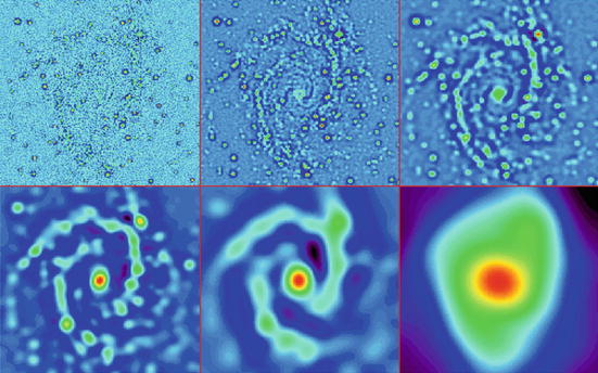
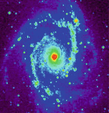
Fig. 3
Wavelet transform of NGC 2997 by the IUWT. The co-addition of these six images reproduces exactly the original image
Fig. 4
Galaxy NGC 2997
The Starlet Reconstruction
The reconstruction is straightforward. A simple co-addition of all wavelet scales reproduces the original map: ![$$c_{0}[k,l] = c_{J}[k,l] +\sum _{ j=1}^{J}w_{j}[k,l]$$](/wp-content/uploads/2016/04/A183156_2_En_34_Chapter_IEq23.gif) . But because the transform is non-subsampled, there are many ways to reconstruct the original image from its wavelet transform [53]. For a given wavelet filter bank (h, g), associated with a scaling function ϕ and a wavelet function ψ, any synthesis filter bank
. But because the transform is non-subsampled, there are many ways to reconstruct the original image from its wavelet transform [53]. For a given wavelet filter bank (h, g), associated with a scaling function ϕ and a wavelet function ψ, any synthesis filter bank  , which satisfies the following reconstruction condition
leads to exact reconstruction. For instance, for isotropic h, if we choose  (the synthesis scaling function
  ), we obtain a filter
  defined by [53]
 If h is a positive filter, then g is also positive. For instance, if
 ![$$h_{\mathrm{1D}} = [1,4,6,4,1]/16$$](/wp-content/uploads/2016/04/A183156_2_En_34_Chapter_IEq28.gif) , then
, then ![$$\tilde{g}_{\mathrm{1D}} = [1,4,22,4,1]/16$$](/wp-content/uploads/2016/04/A183156_2_En_34_Chapter_IEq29.gif) . That is,
. That is,  is positive. This means that
  is no longer related to a wavelet function. The 1D detail synthesis function related to
  is defined by
. But because the transform is non-subsampled, there are many ways to reconstruct the original image from its wavelet transform [53]. For a given wavelet filter bank (h, g), associated with a scaling function ϕ and a wavelet function ψ, any synthesis filter bank , which satisfies the following reconstruction condition(8)
(the synthesis scaling function ), we obtain a filter defined by [53], then . That is, is positive. This means that is no longer related to a wavelet function. The 1D detail synthesis function related to is defined by(9)
Note that by choosing  , any synthesis function
  which satisfies
leads to an exact reconstruction [36] and  can take any value. The synthesis function
  does not need to verify the admissibility condition (i.e., to have a zero mean).
, any synthesis function which satisfies(10)
can take any value. The synthesis function does not need to verify the admissibility condition (i.e., to have a zero mean).


Starlet Transform: Second Generation
A particular case is obtained when  and
and  , which leads to a filter g 1D equal to δ − h 1D ⋆ h 1D. In this case, the synthesis function
  is defined by
  , and the filter
  is the solution to (8).
and , which leads to a filter g 1D equal to δ − h 1D ⋆ h 1D. In this case, the synthesis function is defined by , and the filter is the solution to (8).We end up with a synthesis scheme where only the smooth part is convolved during the reconstruction.
Deriving h from a spline scaling function, for instance ![$$B_{1}(h_{1} = [1,2,1]/4)$$](/wp-content/uploads/2016/04/A183156_2_En_34_Chapter_IEq48.gif) or
or ![$$B_{3}\ (h_{3} = [1,4,6,4,1]/16)$$](/wp-content/uploads/2016/04/A183156_2_En_34_Chapter_IEq49.gif) (note that
(note that  ), since h 1D is even-symmetric (i.e.,
  ), the z-transform of g 1D is then
which is the z-transform of the filter
![$$\displaystyle{g_{\mathrm{1D}} = [-1,-8,-28,-56,186,-56,-28,-8,-1]/256.}$$](/wp-content/uploads/2016/04/A183156_2_En_34_Chapter_Equd.gif)
or (note that ), since h 1D is even-symmetric (i.e., ), the z-transform of g 1D is then(11)
We get the following filter bank:
![$$\displaystyle\begin{array}{rcl} \begin{array}{ll} h_{\mathrm{1D}} & = h_{3} = \tilde{h} = [1,4,6,4,1]/16 \\ g_{\mathrm{1D}} & =\delta -h \star h = [-1,-8,-28,-56,186,-56,-28,-8,-1]/256\\ \tilde{g}_{ \mathrm{1D}} & =\delta .\end{array} & &{}\end{array}$$](/wp-content/uploads/2016/04/A183156_2_En_34_Chapter_Equ12.gif)
(12)
The second-generation starlet transform algorithm is:
1.
We initialize j to 0 and we start with the data c j [k].
2.
We carry out a discrete convolution of the data c j [k] using the filter h 1D. The distance between the central pixel and the adjacent ones is 2 j . We obtain c j+1[k].
3.
We do exactly the same convolution on c j+1[k] and we obtain c j+1 ′ [k].
4.
After this two-step smoothing, we obtain the discrete starlet wavelet transform from the difference ![$$w_{j+1}[k] = c_{j}[k] - c_{j+1}^{{\prime}}[k]$$](/wp-content/uploads/2016/04/A183156_2_En_34_Chapter_IEq52.gif) .
.
.5.
If j is less than the number J of resolutions we want to compute, we increment j and then go to step 2.
6.
The set  represents the starlet wavelet transform of the data.
represents the starlet wavelet transform of the data.As in the standard starlet transform, extension to 2D is trivial. We just replace the convolution with h 1D by a convolution with the filter h 2D, which is performed efficiently by using the separability.
With this specific filter bank, there is a no convolution with the filter  during the reconstruction. Only the low-pass synthesis filter
  is used.
during the reconstruction. Only the low-pass synthesis filter is used.The reconstruction formula is
![$$\displaystyle\begin{array}{rcl} c_{j}[l] = (h_{\mathrm{1D}}^{(j)} \star c_{ j+1})[l] + w_{j+1}[l]\,& &{}\end{array}$$](/wp-content/uploads/2016/04/A183156_2_En_34_Chapter_Equ13.gif)
and denoting  and L 0 = δ, we have
![$$\displaystyle\begin{array}{rcl} c_{0}[l] = \left (L^{J} \star c_{ J}\right )[l] +\sum _{ j=1}^{J}\left (L^{j-1} \star w_{ j}\right )[l].& &{}\end{array}$$](/wp-content/uploads/2016/04/A183156_2_En_34_Chapter_Equ14.gif)
Each wavelet scale is convolved with a low-pass filter.
(13)
and L 0 = δ, we have(14)
The second-generation starlet reconstruction algorithm is:
1.
The set  represents the input starlet wavelet transform of the data.
represents the input starlet wavelet transform of the data.2.
We initialize j to J − 1 and we start with the coefficients c j [k].
3.
We carry out a discrete convolution of the data c j+1[k] using the filter (h 1D). The distance between the central pixel and the adjacent ones is 2 j . We obtain c j+1 ′ [k].
4.
Compute ![$$c_{j}[k] = c_{j+1}^{{\prime}}[k] + w_{j+1}[k]$$](/wp-content/uploads/2016/04/A183156_2_En_34_Chapter_IEq58.gif) .
.
.5.
If j is larger than 0,  and then go to step 3.
and then go to step 3.6.
c 0 contains the reconstructed data.
As for the transformation, the 2D extension consists just in replacing the convolution by h 1D with a convolution by h 2D.
Figure 6 shows the analysis scaling and wavelet functions. The synthesis functions  and
and  are the same as those in Fig. 5. As both are positive, we have a decomposition of an image X on positive scaling functions
  and
and  , but the coefficients α are obtained with the starlet wavelet transform and have a zero mean (except for c J ), as a regular wavelet transform.
and are the same as those in Fig. 5. As both are positive, we have a decomposition of an image X on positive scaling functions and , but the coefficients α are obtained with the starlet wavelet transform and have a zero mean (except for c J ), as a regular wavelet transform.Fig. 6
Left, the ϕ 1D analysis scaling function and right, the ψ 1D analysis wavelet function. The synthesis functions  and
and  are the same as those in Fig. 5
and are the same as those in Fig. 5 In 2D, similarly, the second-generation starlet transform leads to the representation of an image X[k, l]:
![$$\displaystyle\begin{array}{rcl} X[k,l] =\sum _{m,n}\phi _{j,k,l}^{(1)}(m,n)c_{ J}[m,n] +\sum _{ j=1}^{J}\sum _{ m,n}\phi _{j,k,l}^{(2)}(m,n)w_{ j}[m,n]\,& &{}\end{array}$$](/wp-content/uploads/2016/04/A183156_2_En_34_Chapter_Equ15.gif)
where  and
and  .
.
(15)
and .ϕ (1) and ϕ (2) are positive, and w j are zero mean 2D wavelet coefficients.
The advantage of the second-generation starlet transform will be seen in section “Sparse Positive Decomposition” below.
Sparse Modeling of Astronomical Images
Using the sparse modeling, we now consider that the observed signal X can be considered as a linear combination of a few atoms of the wavelet dictionary ![$$\boldsymbol{\Phi } = [\phi _{1},\ldots,\phi _{T}]$$](/wp-content/uploads/2016/04/A183156_2_En_34_Chapter_IEq68.gif) . The model of Eq. 3 is then replaced by the following:
. The model of Eq. 3 is then replaced by the following:
and  , and
, and  . Furthermore, most of the coefficients α will be equal to zero. Positions and scales of active coefficients are unknown, but they can be estimated directly from the data Y. We define the multiresolution support M of an image Y by
![$$\displaystyle\begin{array}{rcl} M_{j}[k,l] = \left \{\begin{array}{ll} \text{ 1 }&\text{ if }w_{j}[k,l]\text{ is significant} \\ \text{ 0 }&\text{ if }w_{j}[k,l]\text{ is not significant} \end{array} \right.& &{}\end{array}$$](/wp-content/uploads/2016/04/A183156_2_En_34_Chapter_Equ17.gif)
where w j [k, l] is the wavelet coefficient of Y at scale j and at position (k, l). Hence, M describes the set of active atoms in Y. If H is compact and not too extended, then M describes also well the active set of X. This is true because the background B is generally very smooth, and therefore, a wavelet coefficient w j [k, l] of Y, which does not belong to the coarsest scale, is only dependent on X and N (the term < ϕ i , B > being equal to zero).
. The model of Eq. 3 is then replaced by the following:(16)
, and . Furthermore, most of the coefficients α will be equal to zero. Positions and scales of active coefficients are unknown, but they can be estimated directly from the data Y. We define the multiresolution support M of an image Y by(17)
Selection of Significant Coefficients Through Noise Modeling
We need now to determine when a wavelet coefficient is significant. Wavelet coefficients of Y are corrupted by noise, which follows in many cases a Gaussian distribution, a Poisson distribution, or a combination of both. It is important to detect the wavelet coefficients which are “significant,” i.e., the wavelet coefficients which have an absolute value too large to be due to noise.
For Gaussian noise, it is easy to derive an estimation of the noise standard deviation σ j at scale j from the noise standard deviation, which can be evaluated with good accuracy in an automated way [55]. To detect the significant wavelet coefficients, it suffices to compare the wavelet coefficients w j [k, l] to a threshold level t j . t j is generally taken equal to K σ j , and K, as noted in Sect. 2, is chosen between 3 and 5. The value of 3 corresponds to a probability of false detection of 0. 27 %. If w j [k, l] is small, then it is not significant and could be due to noise. If w j [k, l] is large, it is significant:
![$$\displaystyle\begin{array}{rcl} \begin{array}{l} \text{ if }\mid w_{j}[k,l]\mid \ \geq \ t_{j}\ \ \text{ then }w_{j}[k,l]\text{ is significant } \\ \text{ if }\mid w_{j}[k,l]\mid \ < t_{j}\ \ \text{ then }w_{j}[k,l]\text{ is not significant }\end{array} & &{}\end{array}$$](/wp-content/uploads/2016/04/A183156_2_En_34_Chapter_Equ18.gif)
(18)
When the noise is not Gaussian, other strategies may be used:
Poisson noise: if the noise in the data Y is Poisson, the transformation [1] acts as if the data arose from a Gaussian white noise model, with σ = 1, under the assumption that the mean value of Y is sufficiently large. However, this transform has some limits, and it has been shown that it cannot be applied for data with less than 20 counts (due to photons) per pixel. So for X-ray or gamma ray data, other solutions have to be chosen, which manage the case of a reduced number of events or photons under assumptions of Poisson statistics.
Gaussian + Poisson noise: the generalization of variance stabilization [40] is
where α is the gain of the detector and g and σ are the mean and the standard deviation of the readout noise.
![$$\displaystyle\begin{array}{rcl} \mathcal{G}(Y [k,l]) = \frac{2} {\alpha } \sqrt{\alpha Y [k, l] + \frac{3} {8}\alpha ^{2} +\sigma ^{2} -\alpha g}& & {}\\ \end{array}$$](/wp-content/uploads/2016/04/A183156_2_En_34_Chapter_Equ19.gif)
Poisson noise with few events using the MS-VST: for images with very few photons, one solution consists in using the Multi-Scale Variance Stabilization Transform (MS-VST) [66]. The MS-VST combines both the Anscombe transform and the starlet transform in order to produce stabilized wavelet coefficients, i.e., coefficients corrupted by a Gaussian noise with a standard deviation equal to 1. In this framework, wavelet coefficients are now calculated by
where
![$$\displaystyle\begin{array}{rcl} \begin{array}{c} \text{Starlet}\\ + \\ \text{MS-VST}\\ \end{array} \left \{\begin{array}{lll} c_{j} & =&\sum _{m}\sum _{n}h_{1{\mathrm{D}}}[m]h_{1{\mathrm{D}}}[n] \\ & &c_{j-1}[k + 2^{j-1}m,l + 2^{j-1}n] \\ w_{j}& =&\mathcal{A}_{j-1}(c_{j-1}) -\mathcal{A}_{j}(c_{j})\end{array} \right.& & {}\end{array}$$](/wp-content/uploads/2016/04/A183156_2_En_34_Chapter_Equ20.gif)
(19) is the VST operator at scale j defined by
where the variance stabilization constants b (j) and e (j) only depend on the filter h 1D and the scale level j. They can all be precomputed once for any given h 1D [66
(20)Related posts:

Stay updated, free articles. Join our Telegram channel

Full access? Get Clinical Tree