Impedance Tomography

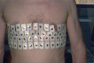
Fig. 1

10-day-old spontaneously breathing neonate lying in the prone position with the head turned to the left. Sixteen medical grade Ag/AgCl electrodes were placed in a transverse plane and connected to a Geo MF-II EIT system [57]

The simplest mathematical formulation of inverse problem of EIT can be stated as follows. Let $\Omega$ be a conducting body described by a bounded domain in $\mathbb{R}^{n}$ , n ≥ 2, with electrical conductivity a bounded and positive function γ(x) (later complex γ will be considered). In the absence of internal sources, the electrostatic potential u in $\Omega$ is governed by the elliptic partial differential equation

$\displaystyle{ L_{\gamma }u:= \nabla \cdot \gamma \nabla u = 0\qquad \text{in}\quad \Omega. }$

(1)

It is natural to consider the weak formulation of (1) in which $u \in H^{1}(\Omega )$ is a weak solution to (1). Given a potential $\phi \in H^{1/2}(\partial \Omega )$ on the boundary, the induced potential $u \in H^{1}(\Omega )$ solves the Dirichlet problem

$\displaystyle{ \left \{\begin{array}{l} L_{\gamma }u = 0\qquad \text{in}\quad \Omega,\\ u\vert _{\partial \Omega } =\phi. \end{array} \right. }$

(2)

The currents and voltages measurements taken on the surface of $\Omega$ , $\partial \Omega$ , are given by the so-called Dirichlet-to-Neumann map (associated with γ) or voltage-to-current map

$\displaystyle{\Lambda _{\gamma }}: u\vert _{\partial \Omega } \in H^{1/2}(\partial \Omega )\longrightarrow \gamma \frac{\partial u} {\partial \nu } \in H^{-1/2}(\partial \Omega ).$

Here, ν denotes the unit outer normal to $\partial \Omega$ and the restriction to the boundary is considered in the sense of the trace theorem on Sobolev spaces. Here, $\partial \Omega$ must be at least Lipschitz continuous and $\gamma \in L^{\infty }(\Omega )$ with $$$\mathrm{ess\,inf\,}\mathrm{Re\,}\gamma = m> 0$$” src=”/wp-content/uploads/2016/04/A183156_2_En_14_Chapter_IEq12.gif”></SPAN>.</DIV><br /> <DIV class=Para>The <SPAN class=EmphasisTypeItalic>forward problem</SPAN> under consideration is the map <SPAN id=IEq13 class=InlineEquation><IMG alt=$ , where $\mathcal{D}_{m} =\{\gamma \in L^{\infty }(\Omega )\vert \mathrm{ess\,inf}\gamma \geq m\}$ The inverse problem for complete data is then the recovery of γ from $\Lambda _{\gamma }$ . As is usual in inverse problems, consideration will be given to questions of (1) uniqueness of solution (or from a practical point of view sufficiency of data), (2) stability/instability with respect to errors in the data, and (3) practical algorithms for reconstruction. It is also worth pointing out to the reader who is not very familiar with EIT the well-known fact that the behavior of materials under the influence of external electric fields is determined not only by the electrical conductivity γ but also by the electric permittivity $\varepsilon$ so that the determination of the complex valued function $\gamma (x,\omega ) =\sigma (x) + {\mathrm{i}}\omega \varepsilon (x)$ would be the more general and realistic problem, where ${\mathrm{i}} = \sqrt{-1}$ and ω is the frequency. The simple case where ω = 0 will be treated in this work. For a description of the formulation of the inverse problem for the complex case, refer for example to [20]. Before addressing questions (1)–(3) mentioned above, it is interesting to consider how the problem arises in practice.

Measurement Systems and Physical Derivation

For the case of direct current, that is the voltage applied is independent of time, the derivation is simple. Of course here $\Omega \subset \mathbb{R}^{3}$ . First suppose that it is possible to apply an arbitrary voltage $\phi \in H^{1/2}(\Omega )$ to the surface. It is typical to assume that the exterior $\mathbb{R}^{3}\setminus \Omega$ is an electrical insulator. An electric potential (voltage) u results in the interior and the current J that flows satisfies the continuum Ohm’s law J = −γ∇u; the absence of current sources in the interior is expressed by the continuum version of Kirchoff’s law ∇⋅ J = 0 which together result in (1). The boundary conditions are controlled or measured using a system of conducting electrodes which are typically applied to the surface of the object. In some applications, especially geophysical, these may be spikes that penetrate the object, but it is common to model these as points on the surface. Most EIT systems are designed to apply a known current on (possibly a subset) or electrodes and measure the voltage that results on electrodes (again possibly a subset, in some cases disjoint from those carrying a nonzero current). In other cases it is a predetermined voltage applied to electrodes and the current measured; there being practical reasons determined by electronics or safety for choosing one over the other. In medical EIT applying known currents and measuring voltages is typical. One reason for this is the desire to limit the maximum current for safety reasons. In practice the circuit that delivers a predetermined current can only do so while the voltage required to do that is within a certain range so both maximum current and voltage are limited. For an electrode (let us say indexed by ℓ) not modeled by a point but covering a region $E_{\ell} \subset \partial \Omega$ the current to that electrode is the integral

$\displaystyle{ I_{\ell} =\int _{E_{\ell}} -\mathbf{J} \cdot \nu \, dx. }$

(3)

Away from electrodes,

$\displaystyle{ \gamma \frac{\partial u} {\partial \nu } = 0,\qquad \mbox{ on }\partial \Omega \setminus \bigcup \limits _{\ell=1}^{L}E_{\ell} }$

(4)

as the air surrounding the object is an insulator. On the conducting electrode, $u\vert _{E_{\ell}} = V _{\ell}$ a constant, or as a differential condition

$\displaystyle{ \nu \times \nabla u = 0\qquad \mbox{ on }\partial \Omega \setminus \bigcup \limits _{\ell=1}^{L}E_{\ell}. }$

(5)

Taken together, (3)–(5) are called the shunt model . This ideal of a perfectly conducting electrode is of course only an approximation. Note that while the condition $u \in H^{1}(\Omega )$ is a sensible condition, which ensures finite total dissipated power, it is not sufficient to ensure (3) is well defined. Indeed for smooth γ and smooth ∂ E _ℓthe condition results in a square root singularity in the current density on the electrode. A more realistic model of electrodes is given later.

It is more common to use alternating current in geophysical and process monitoring applications, and essential in medical applications. Specifically the direction of the current must be reversed within a sufficiently short time to avoid electrochemical effects. This also means that the time average of the applied current should be zero. In medical applications, current in one direction for sufficient duration would result in transport of ions, and one of the effects of this can be stimulation of nerves. It would also degrade electrode behavior due to charge build up and ionic changes in the electrode. As a general rule higher levels of current and voltage are considered safer at higher temporal frequencies. The simplest EIT system therefore operates at a fixed frequency using an oscillator or digital signal processing to produce a sinusoidal current. Measurements are then taken of the magnitude, or in some cases the components that are in phase and π∕2 out of phase with the original sine wave. When an EIT system switches from stimulating one set of electrodes to the next set in a stimululation pattern, the measurements adapt to the new pattern over a finite time, and typical EIT systems are designed to start measuring after this transient term has decayed so as to be negligible.

In geophysics a technique that is complementary to EIT called induced polarization tomography IPT is used to find polarizable minerals. In effect this uses a square wave pulse and measures the transient response [85]. In process tomography a technique known as electrical capacitance tomography is designed for imaging insulating materials with different dielectric permittivities, for example oil and gas in a pipe [60, 101]. Again square waves or pulses are used.

In medical and geophysical problems the response of the materials may vary with frequency. For example in a biological cell higher frequency current might penetrate a largely capacitive membrane and so be influenced by the internal structures of the cell, while lower frequency currents pass around the cell. This has led to electrical impedance tomography spectroscopy (EITS) [47], and in geophysics spectral induced polarization tomography (SIPT) [85]. The spectral response can be established either by using multiple sinusoidal frequencies or by sampling the transient response to a pulse.

Our starting point for the case of alternating current is the time harmonic Maxwell equations at a fixed angular frequency ω. Here it is assumed that the transient components of all fields are negligible and represent the time harmonic electric and magnetics vector fields using the complex representation $\mathcal{F}(x,t) =\mathrm{ Re\,}(\mathbf{F}\exp ({\mathrm{i}}\omega t))$ , yielding

$\displaystyle\begin{array}{rcl} \nabla \times \mathbf{E}& =& -{\mathrm{i}}\omega \mathbf{B},{}\end{array}$

(6)

$\displaystyle\begin{array}{rcl} \nabla \times \mathbf{H}& =& \mathbf{J} + {\mathrm{i}}\omega \mathbf{D}.{}\end{array}$

(7)

The electric and magnetic fields E and H are related to the current density J, electric displacement D, and magnetic flux B by the material properties conductivity σ, permittivity ε, and permeability μ by

$\displaystyle\begin{array}{rcl} \mathbf{J} =\sigma \mathbf{E},\,\mathbf{D} =\epsilon \mathbf{E},\,\mathbf{B} =\mu \mathbf{H}.& &{}\end{array}$

(8)

The fields E and H are evaluated on directed curves, while the “fluxes” J,D and B on surfaces. In biomedical applications one can typically take μ to be constant and to be the same inside the body as outside in air. In non-destructive testing and geophysical applications there may well be materials with differing permeability. Here (8) assumes linear relations. For example the first is the continuum Ohm’s law. Here, the material properties may be frequency dependent. This dispersion is important in EIS and SIPT. For the moment a first approximation is to assume isotropy (so that the material properties are scalars).

There are many inverse problems governed by time harmonic Maxwell’s equations.. These occur at large values of ω and include optical and microwave tomographic techniques and scattering problems such as radar which are not discussed in this chapter. There are also systems where the fields arise from alternating current in a coil, and measurements are made either with electrodes or with other coils. Mutual (or magnetic) induction tomography (MIT) falls into this category and has been tried in medical and process monitoring applications [46]. In these cases the eddy current approximation [9] to Maxwell’s equations is used. While for direct current EIT (i.e., ERT) the object is assumed surrounded by an insulator, in MIT one must account for the magnetic fields in the surrounding space, there being no magnetic “shielding.”

The assumptions used to justify the usual mathematical model of EIT make it distinct from many other inverse problems for Maxwell’s equations. Given

Assumption 1.

Transients components of all fields are negligible .

This assumption simply means that a sufficient “settling time” has been given before making measurements.

The interest in relatively low frequencies, where magnetic effects can be neglected, translates into two assumptions

Assumption 2.

$\omega \sqrt{\epsilon \mu }$ is small compared with the size of $\Omega$ .

This means that the wavelength of propagating waves in the material is large. A measurement accuracy of 2⁻¹² = 1∕4096 is ambitious at higher frequencies means that for wave effects to be negligible

$\displaystyle{ d\,\omega \sqrt{\epsilon \mu } <\cos ^{-1}\frac{4095} {4096}, }$

(9)

where d is the diameter of the body. Taking the relative permittivity to be 10 and R = 0. 3 m gives a maximum frequency of 1 MHz.

Assumption 3.

$\sqrt{ \omega \sigma \mu /2}$ is small compared with the size of $\Omega$ .

The quantity

$\displaystyle{ \delta = \sqrt{\frac{2} {\omega \sigma \mu }} }$

(10)

is known as the skin depth. For a frequency of 10 kHz and a conductivity of 0. 5 Sm⁻¹ typical in medical applications, the skin depth is 7 m. In geophysics lower frequencies are typical but length scales are larger. In a conducting cylinder the electric field decays with distance r from the boundary at a rate e^−r∕δdue to the opposing magnetic field. At EIT frequencies this simple example suggests that accurate forward modeling of EIT should take account of this effect although it is currently not thought to be a dominant source of error.

The effect of Assumptions 2 and 3 combined together is that it is reasonable to neglect ∇× E in Maxwell’s equations resulting in the standard equation for complex EIT

$\displaystyle{ \nabla \cdot (\sigma +{\mathrm{i}}\omega \epsilon )\nabla u = 0. }$

(11)

Here the expression $\gamma =\sigma +{\mathrm{i}}\omega \epsilon$ is called complex conductivity, or logically the admittivity, while 1∕σ is called resistivity and the rarely-used complex 1∕γ impedivity. A scaling argument is given for the approximation (11) in [31], and numerical checks on the validity of the approximation in [37, 104] (Fig. 2).

Fig. 2

A system of electrodes used for chest EIT at Oxford Brookes University. The positions of the electrodes were measured manually with a tape measure and the cross-sectional shape was also determined by manual measurements. These electrodes have a disk of jell containing silver chloride solution that makes contact with the skin. Each electrode was attached to the EIT system by a screened lead, not shown in this picture for clarity

It is often not so explicitly stated but while in the direct current case one can neglect the conductivity of the air surrounding the body, for the alternating current case the electrodes are coupled capacitively and, while σ can be assumed to be zero for air, the permittivity of any material is no smaller than that of a vacuum ε ₀ = 8. 85 × 10⁻¹², although dry air approaches that value. One requires then

Assumption 4.

ωε in the exterior is negligible compared to |σ + i ωε| in the interior .

For example, with a conductivity or 0. 2 Sm⁻¹, the magnitude of the exterior admittivity reaches 2⁻¹² of that value for a frequency of 0.88 MHz. For a more detailed calculation the capacitance between the electrodes externally could be compared with the impedance between electrodes. In ECT frequencies above 1 MHz are used and the exterior capacitance cannot be neglected. Indeed an exterior grounded shield is used so that the exterior capacitive coupling is not affected by the surroundings (see Fig. 3).

Fig. 3

A cross section through a typical ECT sensor around a pipe (internal wall) showing the external screen with radial screens designed to reduce the external capacitive coupling between electrodes

The Concentric Anomaly: A Simple Example

A simple example helps us to understand the instability in the inverse conductivity problem. Let $\Omega$ be the unit disk in $\mathbb{R}^{2}$ with polar coordinates (r, θ) and consider a concentric anomaly in the conductivity of radius ρ < 1

$\displaystyle{ \gamma (x) = \left \{\begin{array}{ll} a_{1},&\vert x\vert \leq \rho \\ a_{0},&\rho <\vert x\vert \leq 1. \end{array} \right. }$

(12)

From separation of variables, matching Dirichlet and Neumann boundary conditions at | x | = ρ, for $n \in \mathbb{Z}$

$\displaystyle{ \Lambda _{\gamma }{\mathrm{e}}^{{\mathrm{i}}n\theta } = \vert n\vert \frac{1 +\mu \rho ^{2\vert n\vert }} {1 -\mu \rho ^{2\vert n\vert }}{\mathrm{e}}^{{\mathrm{i}}n\theta }, }$

(13)

where μ = (a ₁ − a ₀)∕(a ₁ + a ₀). From this one sees the effect of the Dirichlet to Neumann map on the complex Fourier series, and the effect on the real Fourier series is easily deduced. This example was considered in [64] as an example of the eigenvalues and eigenfunctions of $\Lambda _{\gamma }$ , and also by [2] as an example of instability. Thus $\vert \vert \gamma - a_{0}\vert \vert _{L^{\infty }(\Omega )} = \vert a_{1} - a_{0}\vert$ independently of ρ and yet $\Lambda _{\gamma } \rightarrow \Lambda _{a_{0}}$ in the operator norm. Hence if an inverse map $\Lambda _{\gamma }\mapsto \gamma$ exists, it cannot be continuous in this topology. Similar arguments can be used to show instability of inversion in other norms.

This example reveals many other features of the more general problem. For example experimentally one observes saturation: for an object placed away from the boundary, changes in the conductivity of an object with a conductivity close to the background are fairly easily detected, but for an object of very high or low conductivity further changes in conductivity of that object have little effect. This saturation effect was explored for offset circular objects (using conformal mappings) by Seagar [98]. This is also an illustration of the nonlinearity of $\gamma \rightarrow \Lambda _{\gamma }$ . One can also see in this example that smaller objects (with the same conductivity) produce smaller changes in measured data as one might expect.

On the unit circle S ¹ one can define an equivalent norm on the Sobolev space H _◇ ^s(S ¹) (see definitions in the section “The Neumann-to-Dirichlet Map”) by

$\displaystyle{ \left \vert \left \vert \sum \limits _{n=-\infty,n\neq 0}^{\infty }c_{ n}mr{\mathrm{e}}^{{\mathrm{i}}n\theta }\right \vert \right \vert _{ s}^{2} =\sum \limits _{ n=-\infty,n\neq 0}^{\infty }n^{2s}c_{ n}^{2}. }$

(14)

It is clear for this example that $\Lambda _{\gamma }: H_{\diamond}^{s}(S^{1}) \rightarrow H_{\cdot }^{s-1}(S^{1})$ , for any s. Roughly the current is a derivative of potential and one degree of differentiability less smooth. Technically $\Lambda _{\gamma }$ (for any positive $\gamma \in C^{\infty }(\Omega )$ ) is a first order pseudo-differential operator [80]. The observation that for the example ${\mathrm{e}}^{-{\mathrm{i}}n\theta }\Lambda _{\gamma }{\mathrm{e}}^{{\mathrm{i}}n\theta } = \vert n\vert + o(n^{-p})$ as | n | → ∞ for any p > −1 illustrates that the change in conductivity and radius of the interior object is of somewhat secondary importance! In the language of pseudodifferential operators for a general γ such that γ − 1 vanishes in a neighborhood of the boundary, $\Lambda _{\gamma }$ and $\Lambda _{1}$ differ by a smoothing operator.

Since (13), $\Lambda _{\gamma }^{-1}$ is also a well-defined operator on $L_{\cdot }^{2} \rightarrow L_{\cdot }^{2}$ with eigenvalues O( | n | ⁻¹) and is therefore a Hilbert–Schmidt operator. This is also known for the general case [36].

Early work on medical applications of EIT [58, 74] hoped that the forward problem in EIT would be approximated by generalized ray transform – that is integrals along current stream lines. The example of a concentric anomaly was used to illustrate that EIT is nonlocal [99]. If one applies the voltage cos(θ +α), which for a homogeneous disk would result in current streamlines that are straight and parallel, a change in conductivity in a small radius ρ from the center changes all measured currents, not just on lines passing through the region of changed conductivity | x | ≤ ρ. In the 1980s a two-dimensional algorithm that backprojected filtered data along equipotential lines was popularized by Barber and Brown [11]. Berenstein [17] later showed that the linearized EIT problem in a unit disc can be interpreted as the Radon transform with respect to the Poincaré metric and a convolution operator and that Barber and Brown’s algorithm is an approximate inverse to this.

In process applications of EIT and related techniques the term soft field imaging is used, which by analogy to soft field X-rays means a problem that is nonlinear and nonlocal. However in the literature when the “soft field effect” is invoked, it is often not clear if it is the nonlinear or nonlocal aspect to which they refer and, in the authors’ opinion, the term is best avoided.

Measurements with Electrodes

A typical electrical imaging system uses a system of conducting electrodes attached to the surface of the body under investigation. One can apply current or voltage to these electrodes and measure voltage or current respectively. For one particular measurement the voltages (with respect to some arbitrary reference) are V _ℓand the currents I _ℓ, which are arranged in vectors as V and $\mathbf{I} \in \mathbb{C}^{L}\,$ . The discrete equivalent of the Dirichlet-to-Neumann $\Lambda _{\gamma }$ map is the transfer admittance, or mutual admittance matrix Y which is defined by I = YV.

It is easy to see that the vector $\mathbf{1} = (1,1,\ldots,1)^{T}$ is in the null space of Y, and that the range of Y is orthogonal to the same vector. Let S be the subspace of $\mathbb{C}^{L}$ perpendicular to 1; then it can be shown that Y | _Sis invertible from S to S. The generalized inverse (see chapter Linear Inverse Problems) Z = Y ^† is called the transfer impedance. This follows from uniqueness of solution of shunt model boundary value problem.

The transfer admittance , or equivalently transfer impedance, represents a complete set of data which can be collected from the L electrodes at a single frequency for a stationary linear medium. It can be seen from the weak formulation of (11) that Y and Z are symmetric (but for ω ≠ 0 not Hermittian). In electrical engineering this observation is called reciprocity . The dimension of the space of possible transfer admittance matrices is clearly no bigger than L(L − 1)∕2, and so it is unrealistic to expect to recover more unknown parameters than this. In the analogous case of planar resistor networks with L “boundary” electrodes the possible transfer admittance matrices can be characterized completely [33], a characterization which is known at least partly to hold in the planar continuum case [63]. A typical electrical imaging system applies current or voltage patterns which form a basis of the space S, and measures some subset of the resulting voltages which as they are only defined up to an additive constant can be taken to be in S.

The shunt model is nonphysical; in medical application with electrodes applied to skin and in “phantom” tanks used to test EIT systems with ionic solutions in contact with metal electrodes, a contact impedance layer exists between the solution or skin and the electrode. This modifies the shunting effect so that the voltage under the electrode is no longer constant. The voltage on the electrode is still a constant V _ℓso now on E _ℓthere is a voltage drop across the contact impedance layer

$\displaystyle{ \phi +z_{\ell}\sigma \frac{\partial \phi } {\partial \nu } = V _{\ell}, }$

(15)

where the contact impedance z _ℓcould vary over E _ℓbut is usually assumed constant. Experimental studies have shown [56] that a contact impedance on each electrode is required for an accurate forward model. This new boundary condition together with (3) and (4) form the Complete Electrode Model or CEM. For experimental validation of this model see [30], theory [103], and numerical calculations [96, 111]. A nonzero contact impedance removes the singularity in the current density, although high current densities still occur at the edges of the electrodes (Fig. 4). For further details on the singularity in the current density, see [32]. While “point electrodes,” in which the current density is a sum of delta functions, are a limiting case of the CEM, they are not physically realistic as they result in nonphysical potentials not in $H^{1}(\Omega )$ . The trace on the boundary cannot be evaluated at a point, so point measurements of voltage are undefined. However it can be shown that if the conductivity is changed only in the compliment of a neighborhood of $\partial \Omega$ the resulting voltage difference at the boundary can be evaluated at points [52].

Fig. 4

The current density on the boundary with the CEM is greatest at the edge of the electrodes, even for passive electrodes. This effect is reduced as the contact impedance increases. Diagrams courtesy of Andrea Borsic. (a) Current density on the boundary for passive and active electrodes. In fact there is a jump discontinuity at the edge of electrodes for nonzeros contact impedance although the plotting routine has joined the left and right limits. (b) The effect of contact impedance on the potential beneath an electrode. The potential is continuous. (c) Interior current flux near an active electrode. (d) Interior current flux near a passive electrode

The set of imposed current patterns, or excitation patterns, is designed to span S, or at least that part of it that can be accurately measured in a given situation. In medical EIT, with process ERT following suit, early systems designed at Sheffield [11] assumed a two-dimensional circular domain. Identical electrodes were equally spaced on the circumference and, taking them to be numbered anticlockwise, the excitation patterns used were adjacent pairs, that is proportional to

$\displaystyle{ I_{\ell}^{i} = \left \{\begin{array}{ll} 1, &i =\ell\\ - 1, &i =\ell +1 \\ 0, &\mbox{ otherwise }, \end{array} \right. }$

(16)

for i = 1, … L − 1. The electronics behind this is balanced current source connected between two electrodes [59, Chap. 2], and this is somewhat easier to achieve in practice than a variable current source at more than two electrodes. For general geometries, where the electrodes are not placed on a closed curve, other pairs of electrodes are chosen. For example I ₁ ⁱ = −1, while I _ℓⁱ = δ _{i ℓ}, ℓ ≠ 1.

Measurements of voltage can only be differential and so voltage measurements are taken between pairs of electrodes, for example adjacent pairs, or between each and some fixed electrode. In pair drive systems, similar to the original Sheffield system, voltages on electrodes with nonzero currents are not measured, resulting in incomplete knowledge of Z.

In geophysical surface resistivity surveys it is common to use a pair drive and pair measurement system, using electrodes in a line where a two-dimensional approximation is used, or laid out in a rectangular or triangular grid where the full three-dimensional problem is solved. Measurements taken between pairs of non-current carrying electrodes. The choice of measurement strategy is limited by the physical work involved in laying out the cables and by the switching systems. Often electrodes will be distributed along one line and a two-dimensional approximate reconstruction is used as this gives adequate information for less cost. A wider spacing of the current electrodes is used where the features of interest is located at a greater depth below the ground. In another geophysical configuration, cross borehole tomography, electrodes are deployed down several vertical cylindrical holes in the ground, typically filled with water, and current passed between electrodes in the same or between different bore holes. Surface electrodes may be used together with those in the bore holes. In some systems the current is measured to account for a non-ideal current source.

In capacitance tomography a basis of voltage patterns is applied and the choice V _ℓⁱ = δ _{i ℓ}is almost universal. The projection of these vectors to S (denoted as an “electrode-wise basis”) is convenient computationally as a current pattern.

Given a multiple drive system capable of driving an arbitrary vector of currents in S (in practice with in some limits on the maximum absolute current and on the maximum voltage) there remains a choice of excitation patterns. While exact measurements of $\mathbf{Z}\mathbf{I}^{i}$ for I ⁱin any basis for S is clearly sufficient, the situation is more complicated with measurements of finite precision in the presence of noise. If a redundant set of currents is taken, the problem of estimating Z becomes one of multivariate linear regression. The choice of current patterns is then a design matrix. Another approach seeks the minimum set of current patterns that results in usable measurements. Applying each current pattern and taking a set of measurements take a finite time, during which the admittivity changes. Without more sophisticated statistical methods (such as Kalman filters [112]), there are diminishing returns in applying redundant current patterns. Suppose that the total power V ^∗ ZI is constrained (to keep the patient electrically safe) and the current best estimate of the admittivity gives a transfer admittance Z _calc, then it is reasonable to apply currents I such that $(\mathbf{Z} -\mathbf{Z}_{{\mathrm{calc}}})\mathbf{I}$ is above the threshold of voltages that can be accurately measured and modeled. One approach is to choose current patterns that are the right generalized singular vectors of Z −Z _calc with singular values bigger than an error threshold. The generalized singular values are with respect to the norm | | I | | _Z: = | | ZI | | on S and are the extrema of the distinguishability defined as

$\displaystyle{ \frac{\vert \vert (\mathbf{Z} -\mathbf{Z}_{{\mathrm{calc}}})\mathbf{I}\vert \vert } {\vert \vert \mathbf{I}\vert \vert _{\mathbf{Z}}}, }$

(17)

for I ∈ S. These excitation patterns are called “optimal current patterns” [45] and can be calculated from an iterative procedure involving repeated measurement. For circular disk with rotationally symmetric admittivity and equally spaced identical electrodes, the singular vectors will be discrete samples of a Fourier basis and these trigonometric patterns are a common choice for multiple drive systems using a circular array of electrodes.

2 Uniqueness and Stability of the Solution

Uniqueness of solution is very important in inverse problems, although when talking to engineers it is often better to speak of sufficiency of data to avoid confusion. Interestingly it is generally true that results that show insufficiency of data, that one cannot recover an unknown function even if an infinite number of measurements of arbitrary precision are taken, have more impact in applied areas. While there are still unsolved problems in the uniqueness theory for the EIT inverse problem, there has been considerable progress over the last three decades and many important questions have been answered. While for an isotropic real conductivity γ (with certain smoothness assumptions for dimensions n ≥ 3), γ is uniquely determined by the complete data $\Lambda _{\gamma }$ (see [10, 24, 107]), an anisotropic conductivity tensor is not uniquely determined by the boundary data, although some progress on what can be determined in this case has been made (see [3, 6, 43, 79]). Aside from knowing what can and cannot be determined with ideal data, there are two important ways the theoretical work has a practical impact. Firstly in some cases the proof of uniqueness of solution suggests a reconstruction algorithm. As for the two-dimensional case (below) the most effective approach (the so-called $\bar{\partial }$ -method) to uniqueness theory has now been implemented as a fast, practical algorithm. The other is an understanding of the instability and conditional stability of the inverse problem. This helps us to determine what a priori information is helpful in reducing the sensitivity of the solution to errors in the data.

In 1980 Calderón published a paper with the title “On a inverse boundary value problem” [26], where he addressed the problem of whether it is possible to determine the conductivity of a body by making current and voltage measurements at the boundary. It seems that Calderón thought of this problem when he was working as an engineer in Argentina for the Yacimientos Petroliféros Fiscales (YPF), but it was only decades later that he decided to publish his results. This short paper is considered the first mathematical formulation of the problem. For a reprinted version of this manuscript, refer to [27]. The authors wish to recall also the work due to Druskin (see [38–40]) which has been carried on independently from Calderón’s approach and has been devoted to the study of the problem from a geophysical point of view.

The Isotropic Case

Calderón’s Paper

Calderón considered a domain $\Omega$ in $\mathbb{R}^{n}$ , $n \geq 2$ , with Lipschitz boundary $\partial \Omega$ . He took γ be a real bounded measurable function in $\Omega$ with a positive lower bound. Let Q _γbe the quadratic form (associated with $\Lambda _{\gamma }$ ) defined by

$$$\displaystyle{ Q_{\gamma }(\phi ) = \left <\phi,\Lambda _{\gamma }\phi \right> =\int _{\Omega }\gamma \:\vert \nabla u\:\vert ^{2}\:dx, }$$” src=”/wp-content/uploads/2016/04/A183156_2_En_14_Chapter_Equ18.gif”></DIV></DIV><br /> <DIV class=EquationNumber>(18)</DIV></DIV>where <SPAN id=IEq63 class=InlineEquation><IMG alt=$ solves the Dirichlet problem (2). Physically Q _γ(ϕ) is the Ohmic power dissipated when the boundary voltage ϕ is applied. The bilinear form associated with Q _γis then obtained by using the polarization identity

$\displaystyle\begin{array}{rcl} B_{\gamma }(\phi,\:\psi )& =& \frac{1} {2}\bigg\{Q_{\gamma }(\phi +\psi ) - Q_{\gamma }(\phi ) - Q_{\gamma }(\psi )\bigg\} \\ & =& \frac{1} {2}\bigg\{\int _{\Omega }\big(\gamma \vert \nabla (u + v)\vert ^{2} -\gamma \vert \nabla u\vert ^{2} -\gamma \vert \nabla v\vert ^{2}\big)\:dx\bigg\} \\ & =& \int _{\Omega }\gamma \nabla u \cdot \nabla v\:dx, {}\end{array}$

(19)

where L _γv = 0 in $\Omega$ and $v\vert _{\partial \Omega } =\psi \in H^{\frac{1} {2} }(\partial \Omega ).$ Clearly a complete knowledge of any of $\Lambda _{\gamma }$ , Q _γand B _γare equivalent. Calderón considered the “forward” map

$\displaystyle{ \mathbf{Q}:\:\gamma \longrightarrow Q_{\gamma } }$

and proved that Q is bounded and analytic in the subset of $L^{\infty }(\Omega )$ consisting of functions γ which are real and have a positive lower bound. He then investigated the injectivity of the map and in order to do so, he linearized the problem. He in fact proved the injectivity of the Fréchet derivative of Q at γ = 1. Here, a few details of the linearization for a general γ are given. Let u be the solution to (2) and U = u + w satisfy L _γ+δU = 0, with $U\vert _{\partial \Omega } =\phi$ . The perturbation in potential satisfies $w\vert _{\partial \Omega } = 0$ , by considering the Dirichlet data fixed and investigating how the Neumann data varies when γ is perturbed to γ +δ. This yields

$\displaystyle{ L_{\delta }u + L_{\gamma }w + L_{\delta }w = 0. }$

(20)

Now let $G: H^{-1}(\Omega ) \rightarrow H_{0}^{1}(\Omega )$ be the Green’s operator that solves the equivalent of Poisson’s equation for L _γwith zero Dirichlet boundary conditions. That is for $g \in H^{-1}(\Omega )$ , L _γGg = g and $G(g)\vert _{\partial \Omega } = 0$ , the operator equation is given

$\displaystyle{ (1 + GL_{\delta })w = -GL_{\delta }u. }$

(21)

An advantage of using the L ^∞norm is that it is clear $\vert \vert L_{\delta }\vert \vert \rightarrow 0$ in the $H^{1}(\Omega ) \rightarrow H^{-1}(\Omega )$ operator norm as | | δ | | _∞ → 0. This means one can choose δ small enough that | | GL _δ | | < 1 (in the operator norm on $H^{1}(\Omega )$ ) and this ensures that the term in the bracket in (21) is invertible and the operator series in

$\displaystyle{ w = -\left (\sum \limits _{k=1}^{\infty }(-GL_{\delta })^{k}\right )u }$

(22)

is convergent. This proves that the map $\gamma \mapsto u$ and hence Q is not just C ^∞but analytic with (22) its Taylor series. Thus, the linearization of the map $\gamma \mapsto \Lambda _{\gamma }$ is

$\displaystyle{ \Lambda _{\gamma +\delta }\phi = \Lambda _{\gamma }\phi +\gamma \frac{\partial } {\partial \nu }GL_{\delta }u +\delta \frac{\partial u} {\partial \nu } + O(\vert \vert \delta \vert \vert _{\infty }^{2}). }$

(23)

A strength of this argument is that it gives the Fréchet derivative in these norms, rather than just the Gateaux derivative. It is easy to deduce that the Fréchet derivative of Q at γ in the direction δ is given by

$\displaystyle{ d\mathbf{Q}(\gamma )\delta (\phi ) =\int _{\Omega }\delta \vert \nabla u\vert ^{2}\:dx. }$

(24)

In many practical situations it is more common to fix the Neumann boundary conditions and measure the change in boundary voltage as the conductivity changes. Suppose $L_{\gamma }u = 0,L_{\gamma +\delta }U = 0$ , w = U − u with

$\gamma \partial u/\partial \nu = (\gamma +\delta )\partial U/\partial \nu = g \in H_{\cdot }^{-1/2}(\partial \Omega )$

then a similar argument to the above shows

$\displaystyle{ \int _{\partial \Omega }w\gamma \frac{\partial u} {\partial \nu } \:dx = -\int _{\Omega }\delta \vert \nabla u\vert ^{2}\:dx + O(\vert \vert \delta \vert \vert _{ \infty }^{2}). }$

(25)

The polarization identity is often applied to (25) giving

$\displaystyle{ \int _{\partial \Omega }w\gamma \frac{\partial v} {\partial \nu } \,dx = -\int _{\Omega }\delta \nabla u \cdot \nabla v\:dx + O(\vert \vert \delta \vert \vert _{\infty }^{2}), }$

(26)

where L _γv = 0. This is often used in practice with

$\displaystyle{ \gamma \frac{\partial v} {\partial \nu } =\chi _{E_{i}}/\vert E_{i}\vert -\chi _{E_{j}}/\vert E_{j}\vert, }$

(27)

which represents the difference in the characteristic functions of a pair of electrodes. In the case of the shunt model this makes the left-hand side of (25) equal to change that occurs in the difference between voltages on that pair of electrodes when the conductivity is perturbed. The formula (25) and its relatives are referred to as the Geselowitz Sensitivity Theorem in the bioengineering literature. With the CEM (25) still holds, but with u and v satisfying (15) [97].

Returning to Calderón’s argument: for γ = 1 one has L ₁ u = ∇² u. To prove the injectivity of d Q(1) one must show that if the integral appearing in (24) vanishes for all the harmonic functions in $\Omega$ , then $\delta = 0$ in $\Omega$ . Suppose the integral in (24) vanishes for all $u \in H^{1}(\Omega )$ such that $\nabla ^{2}u = 0$ in $\Omega$ , then

$\displaystyle{ \int _{\Omega }\delta \nabla u \cdot \nabla v = 0, }$

(28)

whenever $\nabla ^{2}u = \nabla ^{2}v = 0$ in $\Omega$ . For any $z \in \mathbb{R}^{n}$ consider $a \in \mathbb{R}^{n}$ such that $\vert a\vert =\vert z\vert$ , a ⋅ z = 0 and consider the harmonic functions

$\displaystyle\begin{array}{rcl} & & u(x) = {\mathrm{e}}^{\pi i(z\cdot x)+\pi (a\cdot x)}, \\ & & v(x) = {\mathrm{e}}^{\pi i(z\cdot x)-\pi (a\cdot x)},{}\end{array}$

(29)

which is equivalent to choosing

$\displaystyle{ u(x) = {\mathrm{e}}^{x\cdot \rho },\qquad v(x) = {\mathrm{e}}^{-x\cdot \bar{\rho }}, }$

where $\rho \in \mathbb{C}^{n}$ with

$\displaystyle{ \rho \cdot \rho = 0. }$

Here the real dot product on complex vectors is used ρ ⋅ ρ: = ρ ^Tρ. With the choice made in (29), (28) leads to

$\displaystyle{ 2\pi \vert z\vert ^{2}\int \delta (x){\mathrm{e}}^{2\pi i(z\cdot x)}\:dx = 0,\qquad \mbox{ for:each}\quad z, }$

therefore δ(x) = 0, for all $x \in \Omega$ . Calderón also observed that if the linear operator d Q(1) had a closed range, then one could have concluded that Q itself was injective in a sufficiently small neighborhood of γ=constant. However conditions on the range of d Q(1), that would allow us to use the implicit function theorem, are either false or not known. Furthermore if the range was closed, one could have also concluded that the inverse of d Q(1) was a bounded linear operator by the open mapping theorem. Calderón concluded the paper by giving an approximation for the conductivity γ if

$\displaystyle{ \gamma = 1+\delta }$

and δ is small enough in the L ^∞norm, by making use of the same harmonic functions (29). Calderón’s technique is based on the construction of low frequency oscillating solutions. Sylvester and Uhlmann proved in their fundamental paper [107] a result of uniqueness using high frequencies oscillating solutions of L _γu = 0. Their solutions are of type

$\displaystyle{ u(x,\xi,t) = {\mathrm{e}}^{x\cdot \xi }\:\gamma ^{-\frac{1} {2} }(1 +\psi (x,\xi,t)), }$

which behaves (for high frequencies ξ) in the same way as the solutions used by Calderón. These oscillating solutions have come to be known as complex geometrical optics (CGO) solutions. Before going into more details of the use of CGO solutions, an earlier result using a different approach is given.

Uniqueness at the Boundary

In 1984 Kohn and Vogelius [75] proved that boundary values, and derivatives at the boundary, of a smooth isotropic conductivity γ could be determined from the knowledge of Q _γ. Their result is given by the following theorem.

Theorem 1.

Let $\Omega$ be a domain in $\mathbb{R}^{n}$ (n ≥ 2) with smooth boundary $\partial \Omega$ . Suppose $\gamma _{i} \in C^{\infty }(\bar{\Omega })$ , i = 1,2 is strictly positive and that there is a neighborhood B of some $x^{\star } \in \partial \Omega$ so that

$\displaystyle{ Q_{\gamma _{1}}(f) = Q_{\gamma _{2}}(f),\quad \mbox{ for all }f,\quad f \in H^{\frac{1} {2} }(\partial \Omega ),\quad \text{supp}(f) \subset B. }$

Then

$\displaystyle{ \frac{\partial ^{\vert \alpha \vert }} {\partial x^{\alpha }}\:\gamma _{1}(x^{\star }) = \frac{\partial ^{\vert \alpha \vert }} {\partial x^{\alpha }}\:\gamma _{2}(x^{\star }),\qquad \forall \alpha. }$

Theorem 1 is a local result in the sense that one only need to know Q _γin a open set of the boundary in order to determine the Taylor series of γ on that open set. The global reformulation of this result given in terms of $\Lambda _{\gamma }$ is given below.

Theorem 2.

Let $\gamma _{i} \in C^{\infty }(\bar{\Omega })$ , i = 1,2 be strictly positive. If $\Lambda _{1} = \Lambda _{2}$ , then

$\displaystyle{ \frac{\partial ^{\vert \alpha \vert }} {\partial x^{\alpha }}\:\gamma _{1} = \frac{\partial ^{\vert \alpha \vert }} {\partial x^{\alpha }}\:\gamma _{2},\mbox{ on }\partial \Omega,\qquad \forall \alpha.}$

For a sketch of the proof of Theorem 2 see [110, Sketch of proof of Theorem 4.1, pp 6]. This result settled the identifiability question in the real-analytic category of conductivities. Kohn and Vogelius have extended this result to piecewise real-analytic (e.g., piecewise constant) conductivities in [76]. The proof of this result is based on [75] together with the Runge approximation theorem for solutions of L _γu = 0.

CGO Solutions for the Schrödinger Equation

In 1987 Sylvester and Uhlmann [106, 107] constructed in dimension n ≥ 2 CGO solutions in the whole space for the Schrödinger equation with potential q. Before giving their result, the well-known relation between the conductivity equation and the Schrödinger equation will be derived. This relationship is also important in diffuse optical tomography (see chapter Optical Imaging).

Lemma 1.

Let $\gamma \in C^{2}(\bar{\Omega })$ be strictly positive, yielding

$\displaystyle{ \gamma ^{-\frac{1} {2} }L_{\gamma }(\gamma ^{-\frac{1} {2} }) = \nabla ^{2} - q, }$

(30)

where

$\displaystyle{q = \frac{\nabla ^{2}(\gamma ^{\frac{1} {2} })} {\gamma ^{\frac{1} {2} }}.}$

Proof of Lemma 1.

$\displaystyle{ L_{\gamma }u =\gamma \nabla ^{2}u + \nabla \gamma \cdot \nabla u }$

(31)

therefore

$\displaystyle{ \gamma ^{-\frac{1} {2} }L_{\gamma }u =\gamma ^{\frac{1} {2} }\nabla ^{2}u + \frac{\nabla \ \gamma \cdot \nabla u} {\gamma ^{\frac{1} {2} }}. }$

Consider for $w =\gamma ^{\frac{1} {2} }u$

$\displaystyle\begin{array}{rcl} \nabla ^{2}w - q\:w& =& \nabla ^{2}\left (\gamma ^{\frac{1} {2} }\:u\right ) -\left (\nabla ^{2}\gamma ^{\frac{1} {2} }\right )u {}\\ & =& \nabla \cdot \left (\nabla (\gamma ^{\frac{1} {2} }u)\right ) -\left (\nabla ^{2}\gamma ^{\frac{1} {2} }\right )u {}\\ & =& \nabla \cdot \left ((\nabla \gamma ^{\frac{1} {2} }u) +\gamma ^{\frac{1} {2} }(\nabla u)\right ) -\left (\nabla ^{2}\gamma ^{\frac{1} {2} }\right )u {}\\ & =& (\nabla ^{2}\gamma ^{\frac{1} {2} })u + 2\nabla \gamma ^{\frac{1} {2} } \cdot \nabla u +\gamma ^{\frac{1} {2} }\nabla ^{2}u - (\nabla ^{2}\gamma ^{\frac{1} {2} })u {}\\ & =& \gamma ^{\frac{1} {2} }\nabla ^{2}u + \frac{\nabla \gamma \cdot \nabla u} {\gamma ^{\frac{1} {2} }} {}\\ & =& \gamma ^{-\frac{1} {2} }L_{\gamma }u, {}\\ \end{array}$

which proves (30). □

The term q is usually called the potential of the Schrödinger equation, by analogy with the potential energy in quantum mechanics, this definition being somehow confusing given that in EIT u is the electric potential. The results in [106, 107] state the existence of CGO solutions for the Schrödinger equation with potential q bounded and compactly supported in $\mathbb{R}^{n}$ . This result is as given in [110], which relies on the weighted L ² space $L_{\delta }^{2}(\mathbb{R}^{n}) =\{ f:\int \limits _{\mathbb{R}^{n}}(1 + \vert x\vert ^{2})^{\delta }\vert f(x)\vert ^{2}\,dx\}$ . For δ < 0 this norm controls the “growth at infinity.” The Sobolev spaces $H_{\delta }^{k}(\mathbb{R}^{n})$ are formed in the standard way from $L_{\delta }^{2}(\mathbb{R}^{n})$

$\displaystyle{H_{\delta }^{k}(\mathbb{R}^{n}) =\{ f \in W^{k}(\mathbb{R}^{n})\:\vert \:D^{\alpha }f \in L_{\delta }^{2}(\mathbb{R}^{n}),\quad \text{for all}\:\vert \alpha \vert \leq k\},}$

where α is a multi-index, D ^αf denotes the αth weak derivative of f and $W^{k}(\mathbb{R}^{n})$ is the set of k times weakly differentiable functions on $\mathbb{R}^{n}$ .

Theorem 3.

Let $q \in L^{\infty }(\mathbb{R}^{n})$ , n ≥ 2, with q(x) = 0 for |x|≥ R > 0 and − 1 < δ < 0. Then there exists ε(δ) and such that for every $\rho \in \mathbb{C}^{n}$ satisfying

$\displaystyle{\rho \cdot \rho = 0}$

and

$\displaystyle{\frac{\vert \vert (1 + \vert x\vert ^{2})^{1/2}q\vert \vert _{L^{\infty }(\mathbb{R}^{n})} + 1} {\vert \rho \vert } \leq \epsilon }$

there exists a unique solution to

$\displaystyle{ (\nabla ^{2} - q)u = 0 }$

(32)

of the form

$\displaystyle{ u(x,\rho ) = {\mathrm{e}}^{x\cdot \rho }\left (1 +\psi _{ q}(x,\rho )\right ), }$

(33)

with $\psi _{q}(\cdot,\rho ) \in L_{\delta }^{2}(\mathbb{R}^{n})$ . Moreover $\psi _{q}(\cdot,\rho ) \in H_{\delta }^{2}(\mathbb{R}^{n})$ and for 0 ≤ s ≤ 2 there exists C = C(n,s,δ) > 0 such that

$\displaystyle{ \vert \vert \psi _{q}(\cdot,\rho )\vert \vert _{H^{2}} \leq \frac{C} {\vert \rho \vert ^{1-s}}. }$

(34)

Sketch of the proof of Theorem 3.

Let u be a solution of (32) of type (33), then ψ _qmust satisfy

$\displaystyle{ (\nabla ^{2} + 2\rho \cdot \nabla - q)\psi _{ q} = q. }$

(35)

The idea is that Eq. (35) can be solved for ψ _qby constructing an inverse for (∇² + 2ρ ⋅ ∇) and solving the integral equation

$\displaystyle{ \psi _{q} = (\nabla ^{2} + 2\rho \cdot \nabla )^{-1}\left (q(1 +\psi _{ q})\right ) }$

(36)

for ψ _q. For more details about how to solve the above equation, refer to [110, Lemma 5.2] where it is shown that the integral equation (36) can only be solved in $L_{\delta }^{2}(\mathbb{R}^{n})$ for large | ρ | . □

Other approaches for the construction of CGO solutions for the Schrödinger equation have been considered in [36, 49]. The reader may refer to [110] for more details about references on this topic and a more in-depth explanation about the constructions of this kind of solutions.

Dirichlet-to-Neumann Map and Cauchy Data for the Schrödinger Equation

If 0 is not a Dirichlet eigenvalue for the Schrödinger equation, then the Dirichlet-to-Neumann map associated with a potential q can be defined by

$\displaystyle{ \tilde{\Lambda }_{q}(f)\: =\: \frac{\partial u} {\partial \nu } \vert _{\partial \Omega }, }$

where u solves the Dirichlet problem

$\displaystyle{\left \{\begin{array}{c} (\nabla ^{2} - q)u = 0\quad \text{in}\:\Omega \\ u\vert _{\partial \Omega } = f. \end{array} \right.}$

As a consequence of Lemma 1, for any $q = \frac{\nabla ^{2}\gamma ^{1/2}} {\gamma ^{1/2}}$ ,

$\displaystyle\begin{array}{rcl} \tilde{\Lambda }_{q}(f)& =& \frac{\partial } {\partial \nu }(\gamma ^{\frac{1} {2} }\gamma ^{-\frac{1} {2} }\:u)\vert _{\partial \Omega } {}\\ & =& \Bigg(\frac{\partial \gamma ^{\frac{1} {2} }} {\partial \nu } \:(\gamma ^{-\frac{1} {2} }u) +\gamma ^{\frac{1} {2} }\: \frac{\partial (\gamma ^{-\frac{1} {2} }u)} {\partial \nu } \Bigg)\vert _{\partial \Omega } {}\\ & =& \Bigg(\frac{1} {2}\gamma ^{-\frac{1} {2} }\: \frac{\partial \gamma } {\partial \nu }\:\gamma ^{-\frac{1} {2} } +\gamma ^{\frac{1} {2} }\: \frac{\partial (\gamma ^{-\frac{1} {2} }u)} {\partial \nu } \Bigg)\vert _{\partial \Omega } {}\\ & =& \frac{1} {2}\:\Big(\gamma ^{-1}\frac{\partial \gamma } {\partial \nu }\Big)\vert _{\partial \Omega }\:f +\gamma ^{\frac{1} {2} }\vert _{\partial \Omega }\:\Lambda _{\gamma }\big(\gamma ^{-\frac{1} {2} }\vert _{\partial \Omega }\:f\big). {}\\ \end{array}$

So the two Dirichlet-to-Neumann maps $\tilde{\Lambda }_{q}$ and $\Lambda _{\gamma }$ are related in the following way

$\displaystyle{ \tilde{\Lambda }_{q}(f) = \frac{1} {2}\:\Big(\gamma ^{-1}\frac{\partial \gamma } {\partial \nu }\Big)\vert _{\partial \Omega }\:f +\gamma ^{\frac{1} {2} }\vert _{\partial \Omega }\:\Lambda _{\gamma }\big(\gamma ^{-\frac{1} {2} }\vert _{\partial \Omega }\:f\big), }$

(37)

for any $f \in H^{\frac{1} {2} }(\partial \Omega )$ . For $q \in L^{\infty }(\partial \Omega )$ , the Cauchy data are defined as the set

$\displaystyle{ \mathbf{C_{q}} = \left \{\left (u\vert _{\partial \Omega },\: \frac{\partial u} {\partial \nu } \vert _{\partial \Omega }\right )\:\vert \:u \in H^{1}(\Omega ),\quad (\nabla ^{2} - q)u = 0\quad \mbox{ in}\quad \Omega \right \}. }$

If 0 is not an eigenvalue of ∇² − q, then C _qis the graph given by

$\displaystyle{ \mathbf{C_{q}} = \left \{\left (f,\tilde{\Lambda }_{q}(f)\right ) \in H^{\frac{1} {2} }(\partial \Omega ) \times H^{-\frac{1} {2} }(\partial \Omega )\right \}. }$

The result so far is very general and holds in any dimension n ≥ 2. In the rest of the discussion on the uniqueness of Calderón’s problem, a distinction is made between the higher dimensional case n ≥ 3 and the two-dimensional one.

Global Uniqueness for n ≥ 3

Sylvester and Uhlmann proved in [107] a result of global uniqueness for $C^{2}(\bar{\Omega })$ conductivities by solving in this way the identifiability question with the following result. Their result follows in dimension n ≥ 3 from a more general one for the Schrödinger equation, which is useful in its own right for other inverse problems.

Theorem 4.

Let $q_{i} \in L^{\infty }(\Omega )$ , i=1, 2. Assume $C_{q_{1}} = C_{q_{2}}$ , then q ₁ = q ₂.

Proof of Theorem 4.

This result has been proved by constructing oscillatory solutions of $(\nabla ^{2} - q_{i})\:u_{i} = 0$ in $\mathbb{R}^{n}$ with high frequencies. Beginning with the following equality

$\displaystyle{ \int _{\Omega }(q_{1} - q_{2})u_{1}u_{2} = 0 }$

(38)

is true for any $u_{i} \in H^{1}(\Omega )$ solution to

$\displaystyle{(\nabla ^{2} - q_{ i})u_{i} = 0\qquad \text{in}\quad \Omega,\qquad i = 1,2.}$

Equality (38) follows by

$\displaystyle{\int _{\Omega }(q_{1} - q_{2})u_{1}u_{2} =\int _{\partial \Omega }\left (\frac{\partial u_{1}} {\partial \nu } u_{2} - u_{1}\frac{\partial u_{2}} {\partial \nu } \right )dS,}$

which can be easily obtained by the divergence theorem. This extends q _ion the whole $\mathbb{R}^{n}$ by taking q _i = 0 on $\mathbb{R}^{n}\setminus \Omega$ and taking solutions of

$\displaystyle{(\nabla ^{2} - q_{ i})u_{i} = 0\qquad \text{in}\quad \mathbb{R}^{n},\qquad i = 1,2}$

of the form

$\displaystyle{ u_{i} = {\mathrm{e}}^{x\cdot \rho _{i} }\left (1 +\psi _{q_{i}}(x,\rho _{i})\right ),\qquad i = 1,2, }$

(39)

with | ρ _i | large. This type of solutions are known as CGO solutions. ρ _i, i = 1, 2 is chosen of type

$\displaystyle\begin{array}{rcl} \rho _{1}& =& \frac{\eta } {2} + i\left (\frac{k + l} {2} \right ) \\ \rho _{2}& =& -\frac{\eta } {2} + i\left (\frac{k - l} {2} \right ),{}\end{array}$

(40)

with η, k, $l \in \mathbb{R}^{n}$ and satisfying

$\displaystyle{ \eta \cdot k = k \cdot k =\eta \cdot l = 0,\qquad \vert \eta \vert ^{2} = \vert k\vert ^{2} + \vert l\vert ^{2}, }$

(41)

the choices of η, k, l having been made so that ρ _i⋅ ρ _i = 0, i = 1, 2. With these choices of ρ _i, i = 1, 2,

$\displaystyle\begin{array}{rcl} u_{1}u_{2}& =& \left [{\mathrm{e}}^{x\cdot \frac{\eta }{2} +ix\cdot \left (\frac{k+l} {2} \right )} + {\mathrm{e}}^{x\cdot \frac{\eta }{ 2} +ix\cdot \left (\frac{k+l} {2} \right )}\psi _{q_{ 1}}\right ] {}\\ & & \quad \cdot \left [{\mathrm{e}}^{-x\cdot \frac{\eta }{2} +ix\cdot \left (\frac{k-l} {2} \right )} + {\mathrm{e}}^{-x\cdot \frac{\eta }{ 2} +ix\cdot \left (\frac{k-l} {2} \right )}\psi _{q_{ 2}}\right ] {}\\ & =& {\mathrm{e}}^{ix\cdot k}\left (1 +\psi _{ q_{1}} +\psi _{q_{2}} +\psi _{q_{1}}\psi _{q_{2}}\right ) {}\\ \end{array}$

and therefore

$\displaystyle{ \widehat{(q_{1} - q_{2})}(-k) = -\int _{\Omega }{\mathrm{e}}^{ix\cdot k}(q_{ 1} - q_{2})(\psi _{q_{1}} +\psi _{q_{2}} +\psi _{q_{1}}\psi _{q_{2}})dx. }$

(42)

By recalling that

$\displaystyle{\vert \vert \psi _{q_{i}}\vert \vert _{L^{2}(\Omega )} \leq \frac{C} {\vert \rho _{i}\vert }}$

and letting $\vert l\vert \rightarrow \infty$ one obtains q ₁ = q ₂ (see [110, proof of Theorem 6.2, pp 10]). □

As a consequence of this result, the result [107] stated below is finally obtained.

Theorem 5.

Let $\gamma _{i} \in C^{2}(\bar{\Omega })$ , γ _i strictly positive, i=1, 2. If $\Lambda _{\gamma _{1}} = \Lambda _{\gamma _{2}}$ , then γ ₁ = γ ₂ in $\bar{\Omega }$ .

Theorem 5 has been proved in [107] in a straightforward manner by constructing highly oscillatory solutions to L _γu = 0 in $\Omega$ . In this chapter, the line of [110] is followed in the exposition of such result as a consequence of the more general Theorem 4. Such a choice has been made because of the clearer exposition made in [110].

One can proceed by showing that Theorem 4 implies Theorem 5 for the sake of completeness. The reader can find it also in [110]. The argument used is the following. Let $\gamma _{i} \in C^{2}(\bar{\Omega })$ be strictly positive and $\Lambda _{\gamma _{1}} = \Lambda _{\gamma _{2}}$ . Then by [75],

$\displaystyle\begin{array}{rcl} \gamma _{1}\vert _{\partial \Omega }& =& \gamma _{2}\vert _{\partial \Omega }, {}\\ \frac{\partial \gamma _{1}} {\partial \nu } \vert _{\partial \Omega }& =& \frac{\partial \gamma _{2}} {\partial \nu } \vert _{\partial \Omega }, {}\\ \end{array}$

therefore (37) implies $C_{q_{1}} = C_{q_{2}}$ i.e., q ₁ = q ₂ = : q because of Theorem 4. Recall that

$\displaystyle{q_{i} = \frac{\nabla ^{2}\gamma _{i}^{1/2}} {\gamma _{i}^{1/2}},\qquad i = 1,2,}$

which leads to

$\displaystyle\begin{array}{rcl} \nabla ^{2}\gamma _{ 1}^{\frac{1} {2} } - q\:\gamma _{1}^{\frac{1} {2} }& =& 0 {}\\ \nabla ^{2}\gamma _{ 2}^{\frac{1} {2} } - q\:\gamma _{2}^{\frac{1} {2} }& =& 0 {}\\ \end{array}$

i.e.,

$\displaystyle{ \nabla ^{2}\left (\gamma _{ 1}^{\frac{1} {2} } -\gamma _{2}^{\frac{1} {2} }\right ) -\: q\left (\gamma _{1}^{\frac{1} {2} } -\gamma _{2}^{\frac{1} {2} }\right ) = 0 }$

with

$\displaystyle{ \left (\gamma _{1}^{\frac{1} {2} } -\gamma _{2}^{\frac{1} {2} }\right )\vert _{\partial \Omega }\: =\: 0. }$

Therefore it must be that

$\displaystyle{ \gamma _{1}\: =\:\gamma _{2}\text{in}\quad \Omega, }$

by uniqueness of the solution of the Cauchy problem.

The identifiability question was then pushed forward to the case of $\gamma \in C^{1,\:1}(\bar{\Omega })$ with an affirmative answer by Nachman et al. in 1988 [90]. Nachman extended then this result to domains with C ^1,  1 boundaries (see [88]). The condition on the boundary was relaxed to $\partial \Omega$ Lipschitz by Alessandrini in 1990 in [3]; he proved uniqueness at the boundary and gave stability estimates for $\gamma \in W^{1,\:p}(\Omega )$ , with p > n by making use of singular solutions with an isolated singularity at the center of a ball. This method enables one to construct solutions of L _γu = 0 on a ball behaving asymptotically like the singular solutions of the Laplace–Beltrami equation with separated variables. His results hold in dimension n ≥ 2. Results of global uniqueness in the interior were also found in [3] among piecewise analytic perturbations of γ, giving an extension of Kohn and Vogelius result in [76] to Lipschitz domains.

Going back to the issue of global uniqueness, Brown [22] relaxed the regularity of the conductivity to $\frac{3} {2}+\varepsilon$ derivatives, which was followed by the uniqueness result of Päivärinta et al. [95] for $W^{\frac{3} {2},\infty }$ conductivities. Their result is based on the construction of CGO solutions for conductivities $\gamma \in W^{1,\infty }(\mathbb{R}^{n})$ (n ≥ 2). Recalling in what follows, their construction of the CGO followed by their uniqueness result.

Theorem 6 ([95]).

Let $\gamma \in W^{1,\infty }(\mathbb{R}^{\ltimes })$ , γ strictly positive and γ = 1 outside a large ball. Let − 1 < δ < 0, then for |ρ| sufficiently large there is a unique solution of

$\displaystyle{\mbox{ div}(\gamma \nabla u) = 0\quad \mbox{ in}\quad \mathbb{R}^{\ltimes }}$

of the form

$\displaystyle{ u = {\mathrm{e}}^{x\cdot \rho }\left (\gamma ^{-\frac{1} {2} } +\psi _{\gamma }(x,\rho )\right ), }$

(43)

with $\psi _{\gamma } \in L_{\delta }^{2 }(\mathbb{R}^{n } )$ . Moreover, ψ _γ has the form

$\displaystyle{ \psi _{\gamma }(x,\rho ) = \left (\omega _{0}(x,\rho ) -\gamma ^{-\frac{1} {2} }\right ) +\omega _{1}(x,\rho ), }$

(44)

where ω ₀, ω ₁ satisfy

$\displaystyle{ \lim _{\vert \rho \vert \rightarrow \infty }\vert \vert \omega _{0}(x,\rho ) -\gamma ^{-\frac{1} {2} }\vert \vert _{H_{\delta }^{1}} = 0 }$