Segmentation with Shape Priors: Explicit Versus Implicit Representations

(1)

Department of Computer Science, Technische Universität München, 110 8th Street, Garching, Germany

1 Introduction

Image Analysis and Prior Knowledge

Image segmentation is among the most studied problems in image understanding and computer vision. The goal of image segmentation is to partition the image plane into a set of meaningful regions. Here meaningful typically refers to a semantic partitioning where the computed regions correspond to individual objects in the observed scene. Unfortunately, generic purely low-level segmentation algorithms often do not provide the desired segmentation results, because the traditional low-level assumptions like intensity or texture homogeneity and strong edge contrast are not sufficient to separate objects in a scene.

To overcome these limitations, researchers have proposed to impose prior knowledge into low-level segmentation methods. In the following, we will review methods which allow to impose knowledge about the shape of objects of interest into segmentation processes.

In the literature there exist various definitions of the term shape, from the very broad notion of shape of Kendall [54] and Bookstein [5] where shape is whatever remains of an object when similarity transformations are factored out (i.e., a geometrically normalized version of a gray value image) to more specific notions of shape referring to the geometric outline of an object in 2D or 3D. In this work, we will adopt the latter view and refer to an object’s silhouette or boundary as its shape. Intentionally we will leave the exact mathematical definition until later, as different representations of geometry actually imply different definitions of the term shape.

One can distinguish various kinds of shape knowledge:

Low-level shape priors which typically simply favor shorter boundary length, i.e., curves with shorter boundary have lower shape energy, where boundary length can be measured in various ways [4, 6, 49, 53, 69].
Mid-level shape priors which favor, for example, thin and elongated structures, thereby facilitating the segmentation of roads in satellite imagery or of blood vessels in medical imagery [44, 70, 78].
High-level shape priors which favor similarity to previously observed shapes, such as hand shapes [22, 36, 50], silhouettes of humans [26, 29], or medical organs like the heart, the prostate, the lungs, or the cerebellum [58, 82, 84, 99].

There exists a wealth of works on shape priors for image segmentation. It is beyond the scope of this article to provide a complete overview of existing work. Instead, we will present a range of representative works – with many of the examples taken from the author’s own work – and discuss their advantages and shortcomings. Some of these works are formulated in a probabilistic setting where the challenge is to infer the most likely shape given an image and a set of training shapes. Typically the segmentation is formulated as an optimization problem.

One can distinguish two important challenges:

The modeling challenge: How do we formalize distances between shapes? What probability distributions do we impose? What energies should we minimize?

The algorithmic challenge: How do we minimize the arising cost function? Are the computed solutions globally optimal? If they are not globally optimal, how sensitive are solutions with respect to the initialization?

Explicit Versus Implicit Shape Representation

A central question in the modeling of shape similarity is that of how to represent a shape. Typically one can distinguish between explicit and implicit representations. In the former case, the boundary of the shape is represented explicitly – in a spatially continuous setting, this could be a polygon or a spline curve. In a spatially discrete setting this could be a set of edgles (edge elements) forming a regular grid. Alternatively, shapes can be represented implicitly in the sense that one labels all points in space as being part of the interior or the exterior of the object. In the spatially continuous setting, the optimization of such implicit shape representations is solved by means of partial differential equations. Among the most popular representatives are the level set method [39, 72] or alternative convex relaxation techniques [11]. In the spatially discrete setting, implicit representations have become popular through the graph cut methods [7, 49]. More recently, researchers have also advocated hybrid representations where objects are represented both explicitly and implicitly [90]. Table 1 provides an overview of a few representative works on image segmentation based on explicit and implicit representations of shape.

Table 1

Shapes can be represented explicitly or implicitly, in a spatially continuous or a spatially discrete setting. More recently, researchers have adopted hybrid representations [90], where objects are represented both in terms of their interior (implicitly) and in terms of their boundary (explicitly)

	Spatially continuous	Spatially discrete
Explicit	Polygons [22, 102], splines [3, 36, 53]	Edgel labeling and dyn. progr. [1, 74, 80, 87, 89]	Hybrid repres. and LP relaxation [90]
Implicit	Level set methods [39, 72], convex relaxation [11, 31]	Graph cut methods [6, 49]

Figure 1 shows examples of shape representations using an explicit parametric representation by spline curves (spline control points are marked as black boxes), implicit representations by a signed distance function or a binary indicator function, and an explicit discrete representation (4th image).

Fig. 1

Examples of shape representations by means of a parametric spline curve (1st image), a signed distance function (2nd image), a binary indicator function (3rd image), and an explicit discrete representation (4th image)

As we shall see in the following, the choice of shape representation has important consequences on the class of objects that can be modeled, the type of energy that can be minimized, and the optimality guarantees that can be obtained. Among the goals of this article is to put in contrast various shape representations and discuss their advantages and limitations. In general one observes that:

Implicit representations are easily generalized to shapes in arbitrary dimension. Respective algorithms (level set methods, graph cuts, convex relaxation techniques) straightforwardly extend to three or more dimensions. Instead, the extension of explicit shape representations to higher dimensions is by no means straightforward: The notion of arc-length parameterization of curves does not extend to surfaces. Moreover, the discrete polynomial-time shortest-path algorithms [1, 85, 89] which allow to optimally identify pairwise correspondence of points on either shape do not directly extend to minimal-surface algorithms.
Implicit representations are easily generalized to arbitrary shape topology. Since the implicit representation merely relies on a labeling of space (as being inside or outside the object), the topology of the shape is not constrained. Both level set and graph cut algorithms can therefore easily handle objects of arbitrary topology. Instead, for spatially continuous parametric curves, modeling the transition from a single closed curve to a multiply connected object boundary requires sophisticated splitting and merging techniques [38, 60, 61, 65]. Similarly, discrete polynomial-time algorithms are typically constrained to finding open [1, 20, 23] or closed curves [86, 89].
Explicit boundary representations allow to capture the notion of point correspondence [47, 85, 89]. The correspondence between points on either of two shapes and the underlying correspondence of semantic parts is of central importance to human notions of shape similarity. The determination of optimal point correspondences, however, is an important combinatorial challenge, especially in higher dimensions.
For explicit representations, the modeling of shape similarity is often more straightforward and intuitive. For example, for two shapes parameterized as spline curves, the linear interpolation of these shapes also gives rise to a spline curve and often captures the human intuition of an intermediate shape. Instead, the linear interpolation of implicit representations is generally not straightforward: Convex combinations of binary-valued functions are no longer binary-valued. And convex combinations of signed distance functions are generally no longer a signed distance function. Figure 2 shows examples of a linear interpolations of spline curves and a linear interpolations of signed distance functions. Note that the linear interpolation of signed distance functions may give rise to intermediate silhouettes of varying topology.

Fig. 2

The linear interpolation of spline-based curves (shown here along the first three eigenmodes of a shape distribution) gives rise to a families of intermediate shapes

In the following, we will give an overview over some of the developments in the domain of shape priors for image segmentation. In Sect. 2, we will review a formulation of image segmentation by means of Bayesian inference which allows the fusion of input data and shape knowledge in a single energy minimization framework (Fig. 3). In Sect. 3, we will discuss a framework to impose statistical shape priors in a spatially continuous parametric representation. In Sect. 4, we discuss methods to impose statistical shape priors in level set based image segmentation. In Sect. 5, we discuss statistical models which allow to represent the temporal evolution of shapes and can serve as dynamical priors for image sequence segmentation. And lastly, in Sect. 6, we will present recent developments to impose elastic shape priors in a manner which allows to compute globally optimal shape-consistent segmentations in polynomial time.

Fig. 3

This figure shows the linear interpolation of the signed distance functions associated with two human silhouettes. The interpolation gives rise to intermediate shapes and allows changes of the shape topology. Yet, the linear combination of two signed distance functions is generally no longer a signed distance function

2 Image Segmentation via Bayesian Inference

Over the last decades Bayesian inference has become an established paradigm to tackle data analysis problems – see [30, 105] for example. Given an input image $I: \Omega \rightarrow \mathbb{R}$ on a domain $\Omega \subset \mathbb{R}^{2}$ , a segmentation $\mathcal{C}$ of the image plane $\Omega$ can be computed by maximizing the posterior probability:

$\displaystyle{ \mathcal{P}(\mathcal{C}\,\vert \,I) = \frac{\mathcal{P}(I\,\vert \,\mathcal{C})\;\mathcal{P}(\mathcal{C})} {\mathcal{P}(I)}, }$

(1)

where $\mathcal{P}(I\,\vert \,\mathcal{C})$ denotes the data likelihood for a given segmentation $\mathcal{C}$ and $\mathcal{P}(\mathcal{C})$ denotes the prior probability which allows to impose knowledge about which segmentations are a priori more or less likely.

Maximizing the posterior distribution can be performed equivalently by minimizing the negative logarithm of (1) which gives rise to an energy or cost function of the form

$\displaystyle{ E(\mathcal{C}) = E_{{\mathrm{data}}}(\mathcal{C})\; +\; E_{{\mathrm{shape}}}(\mathcal{C}), }$

(2)

where $E_{{\mathrm{data}}}(\mathcal{C}) = -\log \mathcal{P}(I\,\vert \,\mathcal{C})$ and $E_{{\mathrm{shape}}}(\mathcal{C}) = -\log \mathcal{P}(\mathcal{C})$ are typically referred to as data fidelity term and regularizer or shape prior. By maximizing the posterior, one aims at computing the most likely solution given data and prior. Of course there exist alternative strategies of either computing solutions corresponding to the mean of the distribution rather than its mode or of retaining the entire posterior distribution in order to propagate multiple hypotheses over time, as done, for example, in the context of particle filtering [3].

Over the years various data terms have been proposed. In the following, we will simply use a piecewise-constant approximation of the input intensity I [69]:

$\displaystyle{ E_{{\mathrm{data}}}(\mathcal{C}) =\sum _{ i=1}^{k}\int _{ \Omega _{i}}\big(I(x) -\mu _{i}\big)^{2}dx, }$

(3)

where the regions $\Omega _{1},\mathop{\ldots },\Omega _{k}$ are pairwise disjoint regions separated by the boundary $\mathcal{C}$ and μ _idenotes the average of I over the region $\Omega _{i}$ :

$\displaystyle{ \mu _{i} = \frac{1} {\vert \Omega _{i}\vert }\int _{\Omega _{i}}I(x)\,dx. }$

(4)

More sophisticated data terms based on color likelihoods [8, 57, 103] or texture likelihoods [2, 30] are conceivable.

A glance into the literature indicates that the most prominent image segmentation methods rely on a rather simple geometric shape prior E _shape which energetically favors shapes with shorter boundary length [4, 53, 69], a penalizer which – in a spatially discrete setting – dates back at least as far as the Ising model for ferromagnetism [52]. There are several reasons for the popularity of length constraints in image segmentation. Firstly, solid objects in our world indeed tend to be spatially compact. Secondly, such length constraints are mathematically well studied. They give rise to well-behaved models and algorithms – mean curvature motion in a continuous setting and low-order Markov random fields and submodular cost functions in the discrete setting.

Nevertheless, the preference for a shorter boundary is clearly a very simplistic shape prior. In many applications the user may have a more specific knowledge about what kinds of shapes are likely to arise in a given segmentation task. For example, in biology one may want to segment cells that all have a rather specific size and shape. In medical imaging one may want to segment organs that all have a rather unique shape – up to a certain variability – and preserve a specific spatial relationship with respect to other organs. In satellite imagery one may be most interested in segmenting thin and elongated roads, or in the analysis of traffic scenes from a driving vehicle, the predominant objects may be cars and pedestrians. In the following sections, we will discuss ways to impose such higher-level shape knowledge into image segmentation methods.

3 Statistical Shape Priors for Parametric Shape Representations

Among the most straightforward ways to represent a shape is to model its outline as a parametric curve. An example is a simple closed spline curve $\mathcal{C}\in \mathcal{C}^{k}(\mathbb{S}^{1},\Omega )$ of the form

$\displaystyle{ \mathcal{C}(s) =\sum _{ i=1}^{n}p_{ i}\,B_{i}(s), }$

(5)

where $p_{i} \in \mathbb{R}^{2}$ denote a set of spline control points and B _ia set of spline basis functions of degree k [19, 36, 43, 66]. In the special case of linear basis functions, we simply have a polygonal shape, used, for example, in [102]. With increasing number of control points, we obtain a more and more detailed shape representation – see Fig. 4. It shows one of the nice properties of parametric shape representations: The representation is quite compact in the sense that very detailed silhouettes can be represented by a few real-valued variables.

Fig. 4

Spline representation of a hand shape (left) with increasing resolution

Given a family of m shapes, each represented by a spline curve of a fixed number of n control points, we can think of these training shapes as a set $\{z_{1},\mathop{\ldots },z_{m}\}$ of control point vectors:

$\displaystyle{ z_{i} = (p_{i1},\mathop{\ldots },p_{in}) \in \mathbb{R}^{2n}, }$

(6)

where we assume that all control point vectors are normalized with respect to translation, rotation, and scaling [41].

With this contour representation, the image segmentation problem boils down to computing an optimal spline control point vector $z \in \mathbb{R}^{2n}$ for a given image. The segmentation process can be constrained to familiar shapes by imposing a statistical shape prior computed from the set of training shapes.

Linear Gaussian Shape Priors

Among the most popular shape prior is based on the assumption that the training shapes are Gaussian distributed – see for example [22, 36, 55]. There are several reasons for the popularity of Gaussian distributions. Firstly, according to the central limit theorem, the average of a large number of i.i.d. random variables is approximately Gaussian distributed – so if the observed variations of shape were created by independent processes, then one could expect the overall distribution to be approximately Gaussian. Secondly, the Gaussian distribution can be seen as a second-order approximation of the true distribution. And thirdly, the Gaussian distribution gives rise to a convex quadratic cost function that allows for easy minimization.

In practice, the number of training shapes m is often much smaller than the number of dimensions 2n. Therefore, the estimated covariance matrix $\Sigma$ is degenerate with many zero eigenvalues and thus not invertible. As introduced in [36], a regularized covariance matrix is given by

$\displaystyle{ \Sigma _{\perp } = \Sigma \; +\;\lambda _{\perp }\,\left (I - V \,V ^{t}\right ), }$

(7)

where V is the matrix of eigenvectors of $\Sigma$ . In this way, we replace all zero eigenvalues of the sample covariance matrix $\Sigma$ by a constant λ _⊥ ∈ [0, λ _r], where λ _rdenotes the smallest nonzero eigenvalue of $\Sigma$ . (Note that the inverse $\Sigma _{\perp }^{-1}$ of the regularized covariance matrix defined in (7) fundamentally differs from the pseudoinverse, the former scaling components in degenerate directions by $\lambda _{\perp }^{-1}$ while the latter scaling them by 0.) In [68] it was shown that λ _⊥ can be computed from the true covariance matrix by minimizing the Kullback–Leibler divergence between the exact and the approximated distribution. Yet, since we do not have the exact covariance matrix but merely a sample covariance matrix, the reasoning for determining λ _⊥ suggested in [68] is not justified.

The Gaussian shape prior is then given by

$\displaystyle{ \mathcal{P}(z) = \frac{1} {\vert 2\pi \Sigma _{\perp }\vert ^{1/2}}\exp \left (-\frac{1} {2}\,(z -\bar{ z})^{t}\,\Sigma _{ \perp }^{-1}\,(z -\bar{ z})\right ), }$

(8)

where $\bar{z}$ denotes the mean control point vector.

Based on the Gaussian shape prior, we can define a shape energy that is invariant to similarity transformations (translation, rotation, and scaling) by

$\displaystyle{ E_{{\mathrm{shape}}}(z) = -\log \mathcal{P}\left (\hat{z}\right ), }$

(9)

where $\hat{z}$ is the shape vector upon similarity alignment with respect to the training shapes:

$\displaystyle{ \hat{z} = \frac{R\,(z - z_{0})} {\vert R\,(z - z_{0})\vert }, }$

(10)

where the optimal translation z ₀ and rotation R can be written as functions of z [36]. As a consequence, we can minimize the overall energy

$\displaystyle{ E(z) = E_{{\mathrm{data}}}(C(z))\; +\; E_{{\mathrm{shape}}}(z) }$

(11)

using gradient descent in z. For details on the numerical minimization, we refer to [25, 36].

Figure 5 shows several intermediate steps in a gradient descent evolution on the energy (2) combining the piecewise constant intensity model (3) with a Gaussian shape prior constructed from a set of sample hand shapes. Note how the similarity-invariant shape prior (9) constrains the evolving contour to hand-like shapes without constraining its translation, rotation, or scaling.

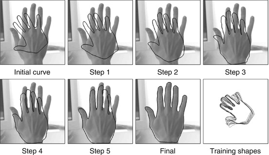
Fig. 5

Evolution of a parametric spline curve during gradient descent on the energy (2) combining the piecewise constant intensity model (3) with a Gaussian shape prior constructed from a set of sample hand shapes (lower right). Note that the shape prior is by construction invariant to similarity transformations. As a consequence, the contour easily undergoes translation, rotation, and scaling as these do not affect the energy

Figure 6 shows the gradient descent evolution with the same shape prior for an input image of a partially occluded hand. Here the missing part of the silhouette is recovered through the statistical shape prior. These evolutions demonstrate that the curve converges to the correct segmentation over rather large spatial distance, an aspect which is characteristic for region-based cost functions like (3).

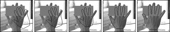
Fig. 6

Gradient descent evolution of a parametric curve from initial to final with similarity-invariant shape prior. The statistical shape prior permits a reconstruction of the hand silhouette in places where it is occluded

Nonlinear Statistical Shape Priors

The shape prior (9) was based on the assumption that the training shapes are Gaussian distributed. For collections of real-world shapes, this is generally not the case. For example, the various silhouettes of a rigid 3D object obviously form a three-dimensional manifold (given that there are only three degrees of freedom in the observation process). Similarly, the various silhouettes of a walking person essentially correspond to a one-dimensional manifold (up to small fluctuations). Furthermore, the manifold of shapes representing deformable objects like human persons are typically very low-dimensional, given that the observed 3D structure only has a small number of joints.

Rather than learning the underlying low-dimensional representation (using principal surfaces or other manifold learning techniques), we can simply estimate arbitrary shape distributions by reverting to nonlinear density estimators – nonlinear in the sense that the permissible shapes are not simply given by a weighted sum of eigenmodes. Classical approaches for estimating nonlinear distributions are the Gaussian mixture model or the Parzen–Rosenblatt kernel density estimator – see Sect. 4.

An alternative technique is to adapt recent kernel learning methods to the problem of density estimation [28]. To this end, we approximate the training shapes by a Gaussian distribution, not in the input space but rather upon transformation $\psi: \mathbb{R}^{2n} \rightarrow Y$ to some generally higher-dimensional feature space Y:

$\displaystyle{ \mathcal{P}_{\psi }(z) \propto \exp \left (-\frac{1} {2}\,(\psi (z) -\psi _{0})^{t}\,\Sigma _{\psi }^{-1}\,(\psi (z) -\psi _{ 0})\right ). }$

(12)

As before, we can define the corresponding shape energy as

$\displaystyle{ E(z) = -\log \mathcal{P}_{\psi }\left (\hat{z}\right ), }$

(13)

with $\hat{z}$ being the similarity-normalized shape given in (10). Here ψ ₀ and $\Sigma _{\psi }$ denote the mean and covariance matrix computed for the transformed shapes:

$\displaystyle{ \psi _{0} = \frac{1} {m}\sum _{i=1}^{m}\psi (z_{ i}),\quad \Sigma _{\psi } = \frac{1} {m}\sum _{i=1}^{m}\,\left (\psi (z_{ i}) -\psi _{0}\right )\left (\psi (z_{i}) -\psi _{0}\right )^{\top }, }$

(14)

where $\Sigma _{\psi }$ is again regularized as in (7).

As shown in [28], the energy E(z) in (13) can be evaluated without explicitly specifying the nonlinear transformation ψ. It suffices to define the corresponding Mercer kernel [24, 67]:

$\displaystyle{ k(x,y):=\langle \psi (x),\psi (y)\rangle \,,\quad \forall x,y \in \mathbb{R}^{2n}, }$

(15)

representing the scalar product of pairs of transformed points ψ(x) and ψ(y). In the following, we simply chose a Gaussian kernel function of width σ:

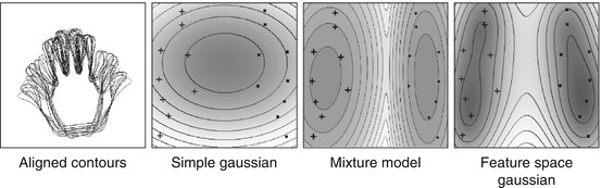
$\displaystyle{ k(x,y) = \frac{1} {(2\pi \sigma ^{2})^{\frac{n} {2} }} \exp \left (-\frac{\vert \vert x - y\vert \vert ^{2}} {2\sigma ^{2}} \right ). }$

(16)

It was shown in [28] that the resulting energy can be seen as a generalization of the classical Parzen–Rosenblatt estimators. In particular, the Gaussian distribution in feature space Y is fundamentally different from the previously presented Gaussian distribution in the input space $\mathbb{R}^{2n}$ . Figure 7 shows the level lines of constant shape energy computed from a set of left- and right-hand silhouettes, displayed in a projection onto the first two eigenmodes of the distribution. While the linear Gaussian model gives rise to elliptical level lines, the Gaussian mixture and the nonlinear Gaussian allow for more general non-elliptical level lines. In contrast to the mixture model, however, the nonlinear Gaussian does not require an iterative parameter estimation process, nor does it require or assume a specific number of Gaussians.

Fig. 7

Model comparison. Density estimates for a set of left ( $\bullet$ ) and right (+) hands, projected onto the first two principal components. From left to right: aligned contours, simple Gaussian, mixture of Gaussians, and Gaussian in feature space (13). In contrast to the mixture model, the Gaussian in feature space does not require an iterative (sometimes suboptimal) fitting procedure

Figure 8 shows screenshots of contours computed for an image sequence by gradient descent on the energy (11) with the nonlinear shape energy (13) computed from a set of 100 training silhouettes. Throughout the entire sequence, the object of interest was occluded by an artificially introduced rectangle. Again, the shape prior allows to cope with spurious background clutter and to restore the missing parts of the object’s silhouette. Two-dimensional projections of the training data and evolving contour onto the first principal components, shown in Fig. 9, demonstrate how the nonlinear shape energy constrains the evolving shape to remain close to the training shapes.

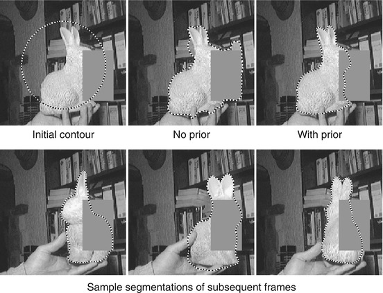
Fig. 8

Tracking a familiar object over a long image sequence with a nonlinear statistical shape prior. A single shape prior constructed from a set of sample silhouettes allows the emergence of a multitude of familiar shapes, permitting the segmentation process to cope with background clutter and partial occlusions

Fig. 9

Tracking sequence from Fig. 8 visualized. Training data ( $\bullet$ ), estimated energy density (shaded), and the contour evolution (white curve) in appropriate 2D projections. The evolving contour – see Fig. 8 – is constrained to the domains of low energy induced by the training data

4 Statistical Priors for Level Set Representations

Parametric representations of shape as those presented above have numerous favorable properties; in particular, they allow to represent rather complex shapes with a few parameters, resulting in low memory requirements and low computation time. Nevertheless, the explicit representation of shape has several drawbacks:

The representation of explicit shapes typically depends on a specific choice of representation. To factor out this dependency in the representation and in respective algorithms gives rise to computationally challenging problems. Determining point correspondences, for example, becomes particularly difficult for shapes in higher dimensions (e.g., surfaces in 3D).
In particular, the evolution of explicit shape representations requires sophisticated numerical regridding procedures to assure an equidistant spacing of control points and prevent control point overlap.
Parametric representations are difficult to adapt to varying topology of the represented shape. Numerically, topology changes require sophisticated splitting and remerging procedures.
A number of recent publications [11, 49, 59] indicate that in contrast to explicit shape representations, the implicit representation of shape allows to compute globally optimal solutions to shape inference for large classes of commonly used energy functionals.

A mathematical representation of shape which is independent of parameterization was pioneered in the analysis of random shapes by Fréchet [45] and in the school of mathematical morphology founded by Matheron and Serra [64, 94]. The level set method [39, 72] provides a means of propagating contours $\mathcal{C}$ (independent of parameterization) by evolving associated embedding functions ϕ via partial differential equations – see Fig. 10 for a visualization of the level set function associated with a human silhouette. It has been adapted to segment images based on numerous low-level criteria such as edge consistency [10, 56, 63], intensity homogeneity [12, 101], texture information [9, 51, 73, 81], and motion information [33].

Fig. 10

The level set method is based on representing shapes implicitly as the zero level set of a higher-dimensional embedding function

In this section, we will give a brief insight into shape modeling and shape priors for implicit level set representations. Parts of the following text were adopted from [34, 35, 82].

Shape Distances for Level Sets

The first step in deriving a shape prior is to define a distance or dissimilarity measure for two shapes encoded by the level set functions ϕ ₁ and ϕ ₂. We shall briefly discuss three solutions to this problem. In order to guarantee a unique correspondence between a given shape and its embedding function ϕ, we will in the following assume that ϕ is a signed distance function, i.e., ϕ > 0 inside the shape, ϕ < 0 outside, and | ∇ϕ | = 1 almost everywhere. A method to project a given embedding function onto the space of signed distance functions was introduced in [98].

Given two shapes encoded by their signed distance functions ϕ ₁ and ϕ ₂, a simple measure of their dissimilarity is given by their L₂-distance in $\Omega$ [62]:

$\displaystyle{ \int \limits _{\Omega }\left (\phi _{1} -\phi _{2}\right )^{2}\,dx. }$

(17)

This measure has the drawback that it depends on the domain of integration $\Omega$ . The shape dissimilarity will generally grow if the image domain is increased – even if the relative position of the two shapes remains the same. Various remedies to this problem have been proposed. We refer to [32] for a detailed discussion.

An alternative dissimilarity measure between two implicitly represented shapes represented by the embedding functions ϕ ₁ and ϕ ₂ is given by the area of the symmetric difference [14, 15, 77]:

$\displaystyle{ d^{2}(\phi _{ 1},\phi _{2}) =\int \limits _{\Omega }\left (H\phi _{1}(x) - H\phi _{2}(x)\right )^{2}\,dx. }$

(18)

In the present work, we will define the distance between two shapes based on this measure, because it has several favorable properties. Beyond being independent of the image size $\Omega$ , measure (18) defines a distance on the set of shapes: it is nonnegative, symmetric, and fulfills the triangle inequality. Moreover, it is more consistent with the philosophy of the level set method in that it only depends on the sign of the embedding function. In practice, this means that one does not need to constrain the two level set functions to the space of signed distance functions. It can be shown [15] that ${\mathrm{L}}^{\infty }$ and W ^1, 2 norms on the signed distance functions induce equivalent topologies as the metric (18).

Since the distance (18) is not differentiable, we will in practice consider an approximation of the Heaviside function H by a smooth (differentiable) version H _ε. Moreover, we will only consider gradients of energies with respect to the L ₂ norm on the level set function, because they are easy to compute and because variations in the signed distance function correspond to respective variations of the implicitly represented curve. In general, however, these do not coincide with the so-called shape gradients – see [46] for a recent work on this topic.

Only gold members can continue reading. Log In or Register to continue