Tomography

” whose value at the point $\left (x,y\right )$ in the section is denoted by $\mu _{\bar{e}}(x,y)$ ) from multiple X-ray projections. A typical method by which data are collected for transverse section imaging in CT is indicated in Fig. 1. A large number of measurements are taken. Each of these measurements is related to an X-ray source position combined with an X-ray detector position, and from the measurements we can (based on physical principles) estimate the line integral of $\mu _{\bar{e}}$ along the line between the source and the detector. The mathematical problem is: given a large number of such projections, reconstruct the image $\mu _{\bar{e}}(x,y)$ .

Fig. 1

Data collection for CT (reproduced from [23])

A chapter such as this can only cover a small part of what is known about tomography. A much extended treatment in the same spirit as this chapter is given in [23]. For additional information on mathematical matters related to CT, the reader may consult the books [7, 17, 24, 29, 50]. In particular, because of the mathematical orientation of this handbook, we will not get into the details of the how the line integrals are estimated from the measurements. (Such details can be found in [23]. They are quite complicated: in addition to the actual measurement with the patient in the scanner a calibration measurement needs to be taken, both of these need to be normalized by the reference detector indicated in Fig. 1, correction has to be made for the beam hardening that occurs due to the X-ray beam being polychromatic rather than consisting of photons at the desired energy $\bar{e}$ , etc.)

2 Background

The problem of image reconstruction from projections has arisen independently in a large number of scientific fields. A most-important version of the problem in medicine is CT; it has revolutionized diagnostic radiology over the past four decades. The 1979 Nobel prize in physiology and medicine was awarded to Allan M. Cormack and Godfrey N. Hounsfield for the development of X-ray computerized tomography [9, 31]. The 1982 Nobel prize in chemistry was awarded to Aaron Klug, one of the pioneers in the use of reconstruction from electron microscopic projections for the purpose of elucidation of biologically important molecular complexes [11, 13]. The 2003 Nobel prize in physiology and medicine was awarded to Paul C. Lauterbur and Peter Mansfield for their discoveries concerning magnetic resonance imaging, which also included the use of image reconstruction from projections methods [38].

In some sense this problem was solved in 1917 by Johann Radon [52]. Let $\ell$ denote the distance of the line L from the origin, let θ denote the angle made with the x axis by the perpendicular drawn from the origin to L (see Fig. 1), and let m(ℓ, θ) denote the integral of $\mu _{\bar{e}}$ along the line L. Radon proved that

$\displaystyle{ \mu _{\bar{e}}(x,y) = -\frac{1} {2\pi ^{2}}\lim _{\varepsilon \rightarrow 0}\int _{\varepsilon }^{\infty }\frac{1} {q}\int _{0}^{2\pi }m_{ 1}(x\cos \theta + y\sin \theta + q,\theta )\,d\theta \,dq, }$

(1)

where m ₁(ℓ, θ) denotes the partial derivative of m(ℓ, θ) with respect to ℓ. The implication of this formula is clear: the distribution of the relative linear attenuation in an infinitely thin slice is uniquely determined by the set of all its line integrals. However:

(a)

Radon’s formula determines an image from all its line integrals. In CT we have only a finite set of measurements; even if they were exactly integrals along lines, a finite number of them would not be enough to determine the image uniquely, or even accurately. Based on the finiteness of the data one can produce objects for which the reconstructions will be very inaccurate (Section 15.4 of [23]).

(b)

The measurements in computed tomography can only be used to estimate the line integrals. Inaccuracies in these estimates are due to the width of the X-ray beam, scatter, hardening of the beam, photon statistics, detector inaccuracies, etc. Radon’s inversion formula is sensitive to these inaccuracies.

(c)

Radon gave a mathematical formula; we need an efficient algorithm to evaluate it. This is not necessarily trivial to obtain. There has been a very great deal of activity to find algorithms that are fast when implemented on a computer and yet produce acceptable reconstructions in spite of the finite and inaccurate nature of the data. This chapter concentrates on this topic.

3 Mathematical Modeling and Analysis

The mathematical model for CT is illustrated in Fig. 1. An engineering realization of this model is shown in Fig. 2. The tube contains a single X-ray source, the detector unit contains an array of X-ray detectors. Suppose for the moment that the X-ray Tube and Collimator on the one side and the Data Acquisition/Detector Unit on the other side are stationary, and the patient on the table is moved between them at a steady rate. By shooting a fan beam of X-rays through the patient at frequent regular intervals and detecting them on the other side, we can build up a two-dimensional X-ray projection of the patient that is very similar in appearance to the image that is traditionally captured on an X-ray film. Such a projection is shown in Fig. 3a. The brightness at a point is indicative of the total attenuation of the X-rays from the source to the detector. This mode of operation is not CT, it is just an alternative way of taking X-ray images. In the CT mode, the patient is kept stationary, but the tube and the detector unit rotate (together) around the patient. The fan beam of X-rays from the source to the detector determines a slice in the patient’s body. The location of such a slice is shown by the horizontal line in Fig. 3a.

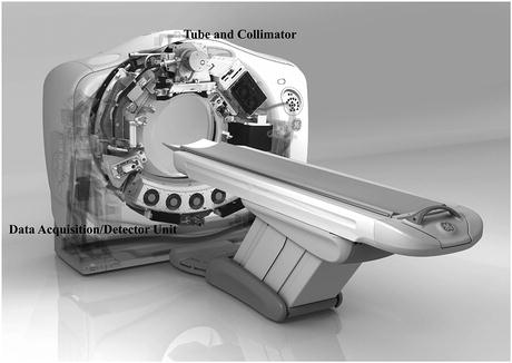
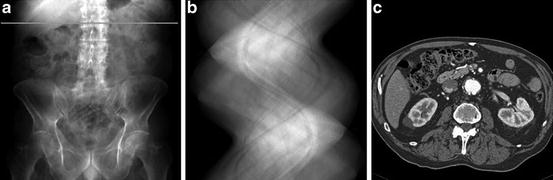
Fig. 2

Engineering rendering of a 2008 CT scanner (provided by GE Healthcare)

Fig. 3

(a) Digitally radiograph with line marking the location of the cross section for which the following images were obtained. (b) Sinogram of the projection data. (c) Reconstruction from the projection data (images were obtained using a Siemens Sensation CT scanner by R. Fahrig and J. Starman at Stanford University)

Data are collected for a number of fixed positions of the source and detector; these are referred to as views. For each view, we have a reading by each of the detectors. All the detector readings for all the views can be represented as a sinogram, shown in Fig. 3b. The intensities in the sinogram are proportional to the line integrals of the X-ray attenuation coefficient between the corresponding source and detector positions. From these line integrals, a two-dimensional image of the X-ray attenuation coefficient distribution in the slice of the body can be produced by the techniques of image reconstruction. Such an image is shown in Fig. 3c. Inasmuch as different tissues have different X-ray attenuation coefficients, boundaries of organs can be delineated and healthy tissue can be distinguished from tumors. In this way CT produces cross-sectional slices of the human body without surgical intervention.

We can use the reconstructions of a series of parallel transverse sections to discover and display the precise shape of selected organs; see Fig. 4. Such displays are obtained by further computer processing of the reconstructed cross sections [59].

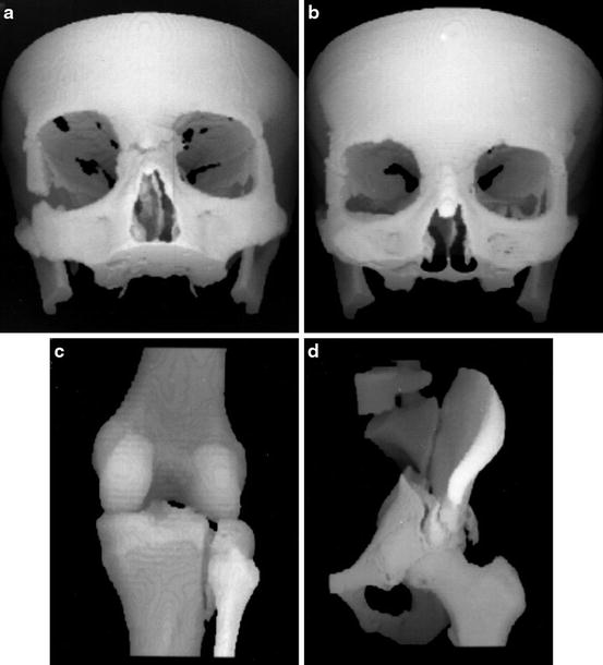
Fig. 4

Three-dimensional displays of bone structures of patients produced during 1986–1988 by software developed in the author’s research group at the University of Pennsylvania for the General Electric Company. (a) Facial bones of an accident victim prior to operation. (b) The same patient at the time of a 1-year postoperative follow-up. (c) A tibial fracture. (d) A pelvic fracture (reproduced from [23])

As a second illustration of the many applications of tomography (for a more complete coverage see Section 1.1 of [23]), we note that three-dimensional reconstruction of nano-scale objects (such as biological macromolecules) can be accomplished using data recorded with a transmission electron microscope (see Fig. 5) that produces electron micrographs, such as the one illustrated in Fig. 6, in which the grayness at each point is indicative of a line integral of a physical property of the object being imaged. From multiple electron micrographs one can recover the structure of the object that is being imaged; see Fig. 7.

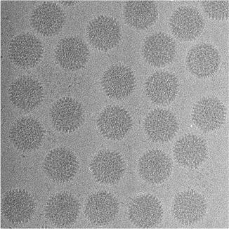
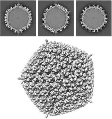
Fig. 5

Schematic drawing of a transmission electron microscope (illustration provided by C. San Martín of the Centro Nacional de Biotecnología, Spain)

Fig. 6

Part of an electron micrograph containing projections of multiple copies of the human adenovirus type 5 (illustration provided by C. San Martín of the Centro Nacional de Biotecnología, Spain)

Fig. 7

Top: Reconstructed values, from electron microscopic data such as in Fig. 6, of the human adenovirus type 5 in three mutually orthogonal slices through the center of the reconstruction. Bottom: Computer graphic display of the surface of the virus based on the three-dimensional reconstruction (illustration provided by C. San Martín of the Centro Nacional de Biotecnología, Spain)

What we have just illustrated in our electron microscopy example is a reconstruction of a three-dimensional object from two-dimensional projections; as opposed to what is shown in Fig. 1, which describes the collection of data for the reconstruction of a two-dimensional object. In fact, recently developed CT scanners are not like that, they collect a series of two-dimensional projections of the three-dimensional object to be reconstructed.

Helical CT (also referred to as spiral CT ) first started around 1990 [10, 34] and has become standard for medical diagnostic X-ray CT . Typical state-of-the-art versions of such systems have a single X-ray source and multiple detectors in a two-dimensional array. The main innovation over previously used technologies is the presence of two independent motions: while the source and detectors rotate around the patient, the table on which the patient lies is continuously moved between them (typically orthogonally to the plane of rotation), see Fig. 8. Thus, the trajectory of the source relative to the patient is a helix (hence the name “helical CT”). Helical CT allows rapid imaging as compared with the previous commercially viable approaches, which has potentially many advantages. One example is when we wish to image a long blood vessel that is made visible to X-rays by the injection of some contrast material: helical CT may very well allow us to image the whole vessel before the contrast from a single injection washes out and this may not be possible by the slower scanning modes. We point out that the CT scanner illustrated in Fig. 2 is in fact modern helical CT scanner.

Fig. 8

Helical (also known as spiral) CT (illustration provided by G. Wang of the Virginia Polytechnic Institute & State University)

For the sake of not over-complicating our discussion, in this chapter we restrict our attention (except where it is explicitly stated otherwise) to the problem of reconstructing two-dimensional objects from one-dimensional projections, rather than to what is done by modern helical cone-beam scanning (as in Fig. 8) and volumetric reconstruction. Schematically, the method of our data collection is shown in Fig. 9. The source and the detector strip are on either side of the object to be reconstructed and they move in unison around a common center of rotation denoted by O in Fig. 9. The data collection takes place in M distinct steps. The source and detector strip are rotated between two steps of the data collection by a small angle, but are assumed to be stationary while the measurement is taken. The M distinct positions of the source during the M steps of the data collection are indicated by the points S ₀, …, S _M−1 in Fig. 9. In simulating this geometry of data collection, we assume that the source is a point source. The detector strip consists of 2N + 1 detectors, spaced equally on an arc whose center is the source position. The line from the source to the center of rotation goes through the center of the central detector. (This description is that of the geometry that is assumed in much of what follows and it does not exactly match the data collection by any actual CT scanner. In particular, in real CT scanners the central ray usually does not go through the middle of the central detector, as a 1/4 detector offset is quite common.) The object to be reconstructed is a picture such that its picture region (i.e., a region outside of which the values assigned to the picture are zero) is enclosed by the broken circle shown in Fig. 9. We assume that the origin of the coordinate system (with respect to which the picture values $\mu _{\bar{e}}(x,y)$ are defined) is the center of rotation, O, of the apparatus.

Fig. 9

Schematic of a standard method of data collection (divergent beam). This is consistent with the data collection mode for CT that is shown in Fig. 1 (reproduced from [23])

Until now we have used $\mu _{\bar{e}}(x,y)$ to denote the relative linear attenuation at the point (x, y), where (x, y) was in reference to a rectangular coordinate system, see Fig. 1. However, it is often more convenient to use polar coordinates. We use the phrase a function of two polar variables to describe a function f whose values f(r, ϕ) represent the value of some physical parameter (such as the relative linear attenuation) at the geometrical point whose polar coordinates are (r, ϕ).

We define the Radon transform $\mathcal{R}f$ of a function f of two polar variables as follows: for any real number pairs (ℓ, θ),

$\displaystyle{ \begin{array}{ccl} \left [\mathcal{R}f\right ](\ell,\theta ) & =&\int _{-\infty }^{\infty }f\left (\sqrt{\ell^{2 } + z^{2}},\,\theta +\tan ^{-1}(z/\ell)\right )dz,\,\,\,\,{\mathrm{if}}\,\,\ell\neq 0,\\ \\ \left [\mathcal{R}f\right ](0,\theta )& =&\int _{-\infty }^{\infty }f\left (z,\theta +\pi /2\right )dz.\end{array} }$

(2)

Observing Fig. 1, we see that $\left [\mathcal{R}f\right ](\ell,\theta )$ is the line integral of f along the line L. (Note that the dummy variable z in (2) does not exactly match the variable z as indicated in Fig. 1. In (2) z = 0 corresponds to the point where the perpendicular dropped on L from the origin meets L.)

In tomography we may assume that a picture function has bounded support; i.e., that there exists a real number E, such that f(r, ϕ) = 0 if r > E. (E can be chosen as the radius of the broken circle in Fig. 9, which should enclose the square-shaped reconstruction region in Fig. 1.) For such a function, $\left [\mathcal{R}f\right ](\ell,\theta ) = 0$ if ℓ > E.

The input data to a reconstruction algorithm are estimates (based on physical measurements) of the values of $\left [\mathcal{R}f\right ](\ell,\theta )$ for a finite number of pairs (ℓ, θ); its output is an estimate, in some sense, of f. Suppose that estimates of $\left [\mathcal{R}f\right ](\ell,\theta )$ are known for I pairs: $\left (\ell_{1},\theta _{1}\right ),\ldots,\ \left (\ell_{I},\theta _{I}\right )$ . For 1 ≤ i ≤ I, we define $\mathcal{R}_{i}f$ by

$\displaystyle{ \mathcal{R}_{i}f = \left [\mathcal{R}f\right ](\ell_{i},\theta _{i}). }$

(3)

In what follows we use y _ito denote the available estimate of $\mathcal{R}_{i}f$ and we use y to denote the I-dimensional vector whose ith component is y _i. We refer to the vector y as the measurement vector . When designing a reconstruction algorithm we assume that the method of data collection, and hence the set $\left \{\left (\ell_{1},\theta _{1}\right ),\ldots,\left (\ell_{I},\theta _{I}\right )\right \}$ , is fixed and known. The reconstruction problem is

$\displaystyle{\mathbf{given}\,\,\text{the data}\,\,y,\,\,\mathbf{estimate}\,\,\text{the picture}\,\,f.}$

We shall usually use f ^∗ to denote the estimate of the picture f.

In the mathematical idealization of the reconstruction problem, what we are looking for is an operator $\mathcal{R}^{-1}$ , which is an inverse of $\mathcal{R}$ in the sense that, for any picture function

, $\mathcal{R}^{-1}\mathcal{R}f$ is

(i.e., $\mathcal{R}^{-1}$ associates with the function $\mathcal{R}f$ the function f). Just as (2) describes how the value of $\mathcal{R}f$ is defined at any real number pair (ℓ, θ) based on the values f assumes at points in its domain, we need a formula that for functions p of two real variables defines $\mathcal{R}^{-1}p$ at points (r, ϕ). Such a formula is

$\displaystyle{ \left [\mathcal{R}^{-1}p\right ](r,\phi ) = \frac{1} {2\pi ^{2}}\int _{0}^{\pi }\int _{ -E}^{E} \frac{1} {r\cos (\theta -\phi )-\ell}p_{1}(\ell,\theta )\,d\ell\,d\theta, }$

(4)

where p ₁(ℓ, θ) denotes the partial derivative of p(ℓ, θ) with respect to ℓ; it is of interest to compare this formula with (1). That the $\mathcal{R}^{-1}$ defined in this fashion is indeed the inverse of $\mathcal{R}$ is proven, for example, in Section 15.3 of [23].

A major category of algorithms for image reconstruction calculate f ^∗ based on (4), or on alternative expressions for the inverse Radon transform $\mathcal{R}^{-1}$ . We refer to this category as transform methods . While (4) provides an exact mathematical inverse, in practice it needs to be evaluated based on finite and imperfect data using the not unlimited capabilities of computers. The essence of any transform method is a numerical procedure (i.e., one that can be implemented on a digital computer), which estimates the value of a double integral, such as the one that appears on the right-hand side of (4), from given values of $y_{i} = p\left (\ell_{i},\theta _{i}\right )$ , 1 ≤ i ≤ I. A very widely used example of transform methods is the so-called filtered backprojection (FBP) algorithm. The reason for this name can be understood by looking at the right-hand side of (4): the inner integral is essentially a filtering of the projection data for a fixed θ and the outer integral backprojects the filtered data into the reconstruction region. However, the implementational details for the divergent beam data collection specified in Fig. 9 are less than obvious, the solution outlined below is based on [28].

The data collection geometry we deal with is also described in Fig. 10. The X-ray source is always on a circle of radius D around the origin. The detector strip is an arc centered at the source. Each line can be considered as one of a set of divergent lines $\left (\sigma,\beta \right )$ , where β determines the source position and σ determines which of the lines diverging from this source position we are considering. This is an alternative way of specifying lines to the (ℓ, θ) notation used previously (in particular in Fig. 1). Of course, each $\left (\sigma,\beta \right )$ line is also an (ℓ, θ) line, for some values of ℓ and θ that depend on σ and β. We use g(σ, β) to denote the line integral of f along the line (σ, β). Clearly,

$\displaystyle{ g(\sigma,\beta ) = \left [\mathcal{R}f\right ](D\sin \sigma,\,\beta +\sigma ). }$

(5)

Fig. 10

Geometry of divergent beam data collection. Every one of the diverging lines is determined by two parameters β and σ. Let O be the origin and S be the position of the source, which always lies on a circle of radius D around O. Then $\beta +\pi /2$ is the angle the line OS makes with the baseline B and σ is the angle the divergent line makes with SO. The divergent line is also one of a set of parallel lines. As such it is determined by the parameters ℓ and θ. Let P be the point at which the divergent line meets the line through O that is perpendicular to it. Then ℓ is the distance from O to P and θ is the angle that OP makes with the baseline (reproduced from [22], Copyright 1981)

As shown in Fig. 9, we assume that projections are taken for M equally spaced values of β with angular spacing $\Delta$ , and that for each view the projected values are sampled at 2N + 1 equally spaced angles with angular spacing λ. Thus g is known at points $(n\lambda,m\Delta ),\,\,-N \leq n \leq N,\,\,0 \leq m \leq M - 1,$ and $M\Delta = 2\pi$ . Even though the projection data consist of estimates (based on measurements) of $g(n\lambda,m\Delta )$ , we use the same notation $g(n\lambda,m\Delta )$ for these estimates. The numerical implementation of the FBP method for divergent beams is carried out in two stages.

First we define, for − N ≤ n ^′ ≤ N,

$\displaystyle\begin{array}{rcl} g_{c}(n^{{\prime}}\lambda,m\Delta )& =& \lambda \sum _{ n=-N}^{N}\cos (n\lambda )g(n\lambda,m\Delta )q^{(1)}\left ((n^{{\prime}}- n)\lambda \right ) \\ & & +\lambda \,\cos (n^{{\prime}}\lambda )\sum _{ n=-N}^{N}g(n\lambda,m\Delta )q^{(2)}\left ((n^{{\prime}}- n)\lambda \right ).{}\end{array}$

(6)

The functions q ⁽¹⁾ and q ⁽²⁾ determine the nature of the “filtering” in the filtered backprojection method. They are not arbitrary, but there are many possible choices for them, for a detailed discussion see Chapter 10 of [23]. Note that the first sum in (6) is a discrete convolution of q ⁽¹⁾ and the projection data weighted by a cosine function, and the second sum is a discrete convolution of q ⁽²⁾ and the projection data.

Second we specify our reconstruction by

$\displaystyle{ f^{{\ast}}(r,\phi ) = \frac{D\Delta } {4\pi ^{2}} \sum _{m=0}^{M-1} \frac{1} {W^{2}}g_{c}\left (\sigma ^{{\prime}},m\Delta \right ), }$

(7)

where

$\displaystyle{ \sigma ^{{\prime}} =\tan ^{-1} \frac{r\cos (m\Delta -\phi )} {D + r\sin (m\Delta -\phi )},\,\,\,\,\,\,\,\,\,-\frac{\pi } {2} \leq \sigma ^{{\prime}}\leq \frac{\pi } {2}, }$

(8)

and

$$$\displaystyle{ W = \left (\left (r\cos (m\Delta -\phi )\right )^{2} + \left (D + r\sin (m\Delta -\phi )\right )^{2}\right )^{1/2},\,\,\,\,\,W > 0. }$$” src=”/wp-content/uploads/2016/04/A183156_2_En_16_Chapter_Equ9.gif”></DIV></DIV><br /> <DIV class=EquationNumber>(9)</DIV></DIV>The meanings of <SPAN class=EmphasisTypeItalic>σ</SPAN> <SUP><SPAN class=EmphasisTypeItalic>′</SPAN> </SUP>and <SPAN class=EmphasisTypeItalic>W</SPAN> are that when the source is at angle <SPAN id=IEq41 class=InlineEquation><IMG alt=$ , the line that goes through (r, ϕ) is $(\sigma ^{{\prime}},m\Delta )$ and the distance between the source and (r, ϕ) is W. Implementation of (7) involves interpolation for approximating $g_{c}(\sigma ^{{\prime}},m\Delta )$ from values of $g_{c}(n^{{\prime}}\lambda,m\Delta )$ . The nature of such an interpolation is discussed in some detail in Section 8.5 of [23]. Note that (7) can be described as a “weighted backprojection.” Given a point (r, ϕ) and a source position $m\Delta$ , the line $(\sigma ^{{\prime}},m\Delta )$ is exactly the line from the source position $m\Delta$ through the point (r, ϕ). The contribution of the convolved ray sum $g_{c}(\sigma ^{{\prime}},m\Delta )$ to the value of f ^∗ at points (r, ϕ) that the line goes through is inversely proportional to the square of the distance of the point (r, ϕ) from the source position $m\Delta$ .

In this chapter we concentrate on the other major category of reconstruction algorithms, the so-called series expansion methods . In transform methods the techniques of mathematical analysis are used to find an inverse of the Radon transform. The inverse transform is described in terms of operators on functions defined over the whole continuum of real numbers. For implementation of the inverse Radon transform on a computer we have to replace these continuous operators by discrete ones that operate on functions whose values are known only for finitely many values of their arguments. This is done at the very end of the derivation of the reconstruction method. The series expansion approach is basically different. The problem itself is discretized at the very beginning: estimating the function is translated into finding a finite set of numbers. This is done as follows.

For any specified picture region, we fix a set of J basis functions $\left \{b_{1},\ldots,b_{J}\right \}$ . These ought to be chosen so that, for any picture f with the specified picture region that we may wish to reconstruct, there exists a linear combination of the basis functions that we consider an adequate approximation to f.

An example of such an approach is the n × n digitization in which we cover the picture region by an n × n array of identical small squares, called pixels . In this case J = n ². We number the pixels from 1 to J, and define

$\displaystyle{ b_{j}(r,\phi ) = \left \{\begin{array}{l} 1,\mbox{ if $(r,\phi )$is inside the $j$th pixel,}\\ 0, \text{ otherwise. } \end{array} \right. }$

(10)

Then the n × n digitization of the picture f is the picture $\hat{f}$ defined by

$\displaystyle{ \hat{f}(r,\phi ) =\sum _{ j=1}^{J}x_{ j}b_{j}(r,\phi ), }$

(11)

where x _jis the average value of f inside the jth pixel. A shorthand notation we use for equations of this type is $\hat{f} =\sum _{ j=1}^{J}x_{j}b_{j}$ .

Another (and usually preferable) way of choosing the basis functions is the following. Generalized Kaiser–Bessel window functions , which are also known by the simpler name blobs , form a large family of functions that can be defined in a Euclidean space of any dimension [40]. Here we restrict ourselves to a subfamily in the two-dimensional plane, whose elements have the form

$\displaystyle{ b_{a,\alpha,\delta }(r,\phi ) = \left \{\begin{array}{@{}l@{\quad }l@{}} C_{a,\alpha,\delta }\left (1 -\left (\frac{r} {a}\right )^{2}\right )I_{ 2}\left (\alpha \sqrt{1 - \left (\frac{r} {a}\right )^{2}}\right ),\quad &\text{if}\;0 \leq r \leq a, \\ 0, \quad &\text{otherwise, } \end{array} \right. }$

(12)

where I _kdenotes the modified Bessel function of the first kind of order k, a stands for the nonnegative radius of the blob, and α is a nonnegative real number that controls the shape of the blob. The multiplying constant C _{a, α, δ}is defined below. Note that such a blob is circularly symmetric, since its value does not depend on ϕ. It has the value zero for all r ≥ a and its first derivatives are continuous everywhere. The “smoothness” of blobs can be controlled by the choice of the parameters a, α and δ, they can be made very smooth indeed as shown in Fig. 11.

Fig. 11

(a) A 243 × 243 digitization of a blob. (b) Its values on the central row (reproduced from [23])

For now let us consider the parameters a, α and δ, and hence the function b _{a, α, δ}, to be fixed. This fixed function gives rise to a set of J basis functions $\left \{b_{1},\ldots,b_{J}\right \}$ as follows. We define a set $G = \left \{g_{1},\ldots,g_{J}\right \}$ of grid points in the picture region. Then, for 1 ≤ j ≤ J, b _jis obtained from b _{a, α, δ}by shifting it in the plane so that its center is moved from the origin to g _j. This definition leaves a great deal of freedom in the selection of G, but it was found in practice advisable that it should consist of those points of a set (in rectangular coordinates)

$\displaystyle{ G_{\delta } = \left \{\left.\left (\frac{m\delta } {2}, \frac{\sqrt{3}n\delta } {2} \right )\right \vert m\text{ and }n\text{ are integers and }m + n\text{ is even}\right \} }$

(13)

that are also in the picture region. Here δ has to be a positive real number and G _δis referred to as the hexagonal grid with sampling distance δ. Having fixed δ, we complete the definition in (12) by

$\displaystyle{ C_{a,\alpha,\delta } = \frac{\sqrt{3}\delta ^{2}\alpha } {4\pi a^{2}I_{3}(\alpha )}. }$

(14)

Pixel-based basis functions (10) have a unit value inside the pixels and zero outside. Blobs, on the other hand, have a bell-shaped profile that tapers smoothly in the radial direction from a high value at the center to the value 0 at the edge of their supports (i.e., at r = a in (12)); see Fig. 11. The smoothness of blobs suggests that reconstructions of the form (11) are likely to be resistant to noise in the data. This has been shown to be particularly useful in fields in which the projection data are noisy, such as positron emission tomography and electron microscopy.

For blobs to achieve their full potential, the selection of the parameters a, α, and δ is important. When they are properly chosen [46], one can approximate homogeneous regions very well, in spite of the bell-shaped profile of the individual blobs. This is illustrated in Fig. 12b, in which a bone cross section shown in Fig. 12a is approximated by a linear combination of blob basis functions with the parameters a = 0. 1551, α = 11. 2829, and δ = 0. 0868. There are some inaccuracies very near the sharp edges, but the interior of the bone is approximated with great accuracy. However, if we change the parameters ever so slightly to a = 0. 16, α = 11. 28, and δ = 0. 09, then the best approximation that can be obtained by a linear combination of blob basis functions is shown in Fig. 12c, which is clearly inferior.

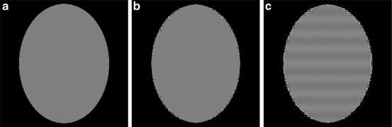
Fig. 12

(a) A 243 × 243 digitization of a bone cross section. (b) Its approximation with default blob parameters and (c) with slightly different parameters. The display window is very narrow for better indication of errors (reproduced from [23])

Irrespective of how the basis functions have been chosen, any picture $\hat{f}$ that can be represented as a linear combination of the basis functions b _jis uniquely determined by the choice of the coefficients x _j, 1 ≤ j ≤ J, in the formula (11). We use x to denote the vector whose jth component is x _jand refer to x as the image vector.

It is easy to see that, under some mild mathematical assumptions,

$\displaystyle{ \mathcal{R}_{i}f \simeq \mathcal{R}_{i}\hat{f} =\sum _{ j=1}^{J}x_{ j}\mathcal{R}_{i}b_{j}, }$

(15)

for 1 ≤ i ≤ I. Since the $b_{j}$ are user-defined, usually the $\mathcal{R}_{i}b_{j}$ can be easily calculated by analytical means. For example, in the case when the b _jare defined by (10), $\mathcal{R}_{i}b_{j}$ is just the length of intersection with the jth pixel of the line of the ith position of the source-detector pair. We use r _i, jto denote our calculated value of $\mathcal{R}_{i}b_{j}$ . Hence,

$\displaystyle{ r_{i,j} \simeq \mathcal{R}_{i}b_{j}. }$

(16)

Recall that y _idenotes the physically obtained estimate of $\mathcal{R}_{i}f.$ Combining this with (15) and (16), we get that, for 1 ≤ i ≤ I,

$\displaystyle{ y_{i} \simeq \sum _{j=1}^{J}r_{ i,j}x_{j}. }$

(17)

Let R denote the matrix whose (i, j)th element is r _i, j. We refer to this matrix as the projection matrix. Let e be the I-dimensional column vector whose ith component, e _i, is the difference between the left- and right-hand sides of (17). We refer to this as the error vector. Then (17) can be rewritten as

$\displaystyle{ y = Rx + e. }$

(18)

The series expansion approach leads us to the following discrete reconstruction problem: based on (18),

$\displaystyle{\mathbf{given}\,\,\text{the data}\,\,y,\,\,\mathbf{estimate}\,\,\text{the image vector}\,\,x.}$

If the estimate that we find as our solution to the discrete reconstruction problem is the vector x ^∗, then the estimate f ^∗ to the picture to be reconstructed is given by

$\displaystyle{ f^{{\ast}} =\sum _{ j=1}^{J}x_{ j}^{{\ast}}b_{ j}. }$

(19)

In (18), the vector e is unknown. The simple approach of trying to solve (18) by first assuming that e is the zero vector is dangerous: y = Rx may have no solutions, or it may have many solutions, possibly none of which is any good for the practical problem at hand. Some criteria have to be developed, indicating which x

Only gold members can continue reading. Log In or Register to continue