for the squared domain (0, 1)2. Images are simultaneously considered as matrices or functions on Ω: A discrete image is an N × N-matrix  . Each of the entries of the matrix represents an intensity value at a pixel. Therewith is associated a piecewise constant function

(1)
![$$\displaystyle{\Omega _{\mathit{ij}}:= \left (\frac{i - 1} {N}, \frac{i} {N}\right ] \times \left (\frac{j - 1} {N}, \frac{j} {N}\right ]\;\text{for}\;1 \leq i,j \leq N,}$$](/wp-content/uploads/2016/04/A183156_2_En_4_Chapter_Equa.gif)
 is the characteristic function of
  . In the context of image processing, U ij denotes the pixel intensity at the pixel
  . A continuous image is a function
  .
.
We emphasize that the measures for comparing images, presented below, can be applied in a straightforward way to higher-dimensional domains, for example, voxel data. However, here, for the sake of simplicity of notation and readability, we restrict attention to a two-dimensional squared domain Ω. Even more, we restrict attention to intensity data and do not consider vector-valued data, such as color images or tensor data. By this restriction, we exclude, for instance, feature-based intensity measures.
2 Distance Measures
In the following, we review distance measures for comparing discrete and continuous images. We review the standard and a morphological distance measure; both of them are deterministic. Moreover, based on the idea to consider images as random variable, we consider in the last two subsections two statistical approaches.
Deterministic Pixel Measure
The most widely used distance measures for discrete and continuous images are the l p , L p distance measures, respectively, in particular p = 2; see, for instance, the chapter Linear Inverse Problems in this handbook. There, two discrete images U 1 and U 2 are similar, if
 respectively, is small. Two continuous images
  are similar if
 is small. Here, ess sup denotes the essential supremum.

 are similar if
Morphological Measures
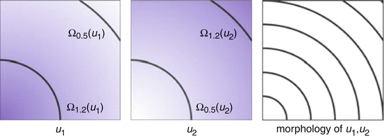
In this subsection, we consider continuous images ![$$u_{i}:\ \varOmega \rightarrow [0,\ 255],\ i = 1,\ 2$$](/wp-content/uploads/2016/04/A183156_2_En_4_Chapter_IEq8.gif) . u 1 and u 2 are morphologically equivalent (Fig. 1), if there exists a one-to-one gray value transformation
. u 1 and u 2 are morphologically equivalent (Fig. 1), if there exists a one-to-one gray value transformation ![$$\upbeta:\ [0,\ 255] \rightarrow [0,\ 255]$$](/wp-content/uploads/2016/04/A183156_2_En_4_Chapter_IEq9.gif) , such that
, such that
 Level sets of a continuous function u are defined as

![$$u_{i}:\ \varOmega \rightarrow [0,\ 255],\ i = 1,\ 2$$](/wp-content/uploads/2016/04/A183156_2_En_4_Chapter_IEq8.gif) . u 1 and u 2 are morphologically equivalent (Fig. 1), if there exists a one-to-one gray value transformation
. u 1 and u 2 are morphologically equivalent (Fig. 1), if there exists a one-to-one gray value transformation ![$$\upbeta:\ [0,\ 255] \rightarrow [0,\ 255]$$](/wp-content/uploads/2016/04/A183156_2_En_4_Chapter_IEq9.gif) , such that
, such that


Fig. 1
The gray values of the images are completely different, but the images u 1, u 2 have the same morphology
The level sets ![$$\varOmega _{\mathbb{R}}(u):=\{\varOmega _{t}(u):\ t \in [0,\ 255]\}$$](/wp-content/uploads/2016/04/A183156_2_En_4_Chapter_IEq10.gif) form the objects of an image that remain invariant under gray value transformations. The normal field (Gauss map) is given by the normals to the level lines and can be written as
form the objects of an image that remain invariant under gray value transformations. The normal field (Gauss map) is given by the normals to the level lines and can be written as
 Droske and Rumpf [7] consider images as similar, if intensity changes occur at the same locations. Therefore, they compare the normal fields of the images with the similarity measure

where they choose the function  appropriately. The vectors
  form an angle that is minimal if the images are morphologically equivalent. Therefore, an appropriate choice of the function g is an increasing function of the minimal angle between v 1, v 2, and
  . For instance, setting g to be the cross or the negative dot product, we obtain
 (The vectors n have to be embedded in
  in order to calculate the cross product.)
![$$\varOmega _{\mathbb{R}}(u):=\{\varOmega _{t}(u):\ t \in [0,\ 255]\}$$](/wp-content/uploads/2016/04/A183156_2_En_4_Chapter_IEq10.gif) form the objects of an image that remain invariant under gray value transformations. The normal field (Gauss map) is given by the normals to the level lines and can be written as
form the objects of an image that remain invariant under gray value transformations. The normal field (Gauss map) is given by the normals to the level lines and can be written as

(2)
 appropriately. The vectors
  form an angle that is minimal if the images are morphologically equivalent. Therefore, an appropriate choice of the function g is an increasing function of the minimal angle between v 1, v 2, and
  . For instance, setting g to be the cross or the negative dot product, we obtain
 in order to calculate the cross product.)
Example 1.
Consider the following scaled images ![$$u_{i}\:\ [0,\ 1]^{2} \rightarrow [0,\ 1]$$](/wp-content/uploads/2016/04/A183156_2_En_4_Chapter_IEq15.gif) ,
,
 with gradients
 With
With  , the functional
  defined in (2) attains the following values for the particular images:
 The similarity measure indicates that u 1 and u 2 are morphologically identical.
![$$u_{i}\:\ [0,\ 1]^{2} \rightarrow [0,\ 1]$$](/wp-content/uploads/2016/04/A183156_2_En_4_Chapter_IEq15.gif) ,
,

 , the functional
  defined in (2) attains the following values for the particular images:
The normalized gradient field is set valued in regions where the function is constant. Therefore, the numerical evaluation of the gradient field is highly unstable. To overcome this drawback, Haber and Modersitzki [15] suggested to use regularized normal gradient fields:
 where
where  for every
  . The parameter ε is connected to the estimated noise level in the image. In regions where ε is much larger than the gradient, the regularized normalized fields n ε (u) are almost zero and therefore do not have a significant effect of the measures
  or
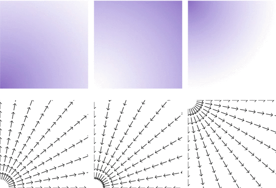
or  , respectively. However, in regions where ε is much smaller than the gradients, the regularized normal fields are close to the non-regularized ones (Fig. 2).

 for every
  . The parameter ε is connected to the estimated noise level in the image. In regions where ε is much larger than the gradient, the regularized normalized fields n ε (u) are almost zero and therefore do not have a significant effect of the measures
  or
or  , respectively. However, in regions where ε is much smaller than the gradients, the regularized normal fields are close to the non-regularized ones (Fig. 2).
Fig. 2
Top: images u 1, u 2, u 3. Bottom: n(u 1), n(u 2), n(u 3)
Statistical Distance Measures
Several distance measures for pairs of images can be motivated from statistics by considering the images as random variables. In the following, we analyze discrete images from a statistical point of view. For this purpose, we need some elementary statistical definitions. Applications of the following measures are mentioned in section “Morphological Measures”:
Correlation Coefficient:
 denote the mean intensity and variance of the discrete image U.


 is close to one, then it indicates that U 1 and U 2 are linearly dependent.
Correlation Ratio: In statistics, the correlation ratio is used to measure the relationship between the statistical dispersion within individual categories and the dispersion across the whole population. The correlation ratio is defined by
 where
where  is the conditional expectation of U 2 subject to U 1.

 is the conditional expectation of U 2 subject to U 1.
To put this into the context of image comparison, let
 be the discrete level set of intensity t ∈ {0, …, 255}. Then the expected value of U 2 on the t-th level set of U 1 is given by
 where
where  denotes the number of pixels in U 1 with gray value t. Moreover, the according conditional variance is defined by
 The function
 is called the discrete histogram of U 1.


 denotes the number of pixels in U 1 with gray value t. Moreover, the according conditional variance is defined by

The correlation ratio is nonsymmetric, that is,  , and takes values in [0, 1]. It is a measure of (non)linear dependence between two images. If
  , then the correlation ratio is maximal.
 , and takes values in [0, 1]. It is a measure of (non)linear dependence between two images. If
  , then the correlation ratio is maximal.
Variance of Intensity Ratio, Ratio Image Uniformity: This measure is based on the definition of similarity that two images are similar, if the factor  has a small variance. The ratio image uniformity (or normalized variance of the intensity ratio) can be calculated by
 It is not symmetric.
 has a small variance. The ratio image uniformity (or normalized variance of the intensity ratio) can be calculated by
Example 2.
Consider the discrete images U 1, U 2, and U 3 in Fig. 3. Table 1 shows a comparison of the different similarity measures. The variance of the intensity ratio is insignificant and therefore cannot be used to determine similarities. The correlation ratio is maximal for the pairing U 1, U 2, and in fact there is a functional dependence of the intensity values of U 1 and U 2. However, the dependence of the intensity values of U 1 and U 2 is nonlinear; hence, the absolute value of the correlation coefficient (measure of linear dependence) is close to one, but not identical to one.
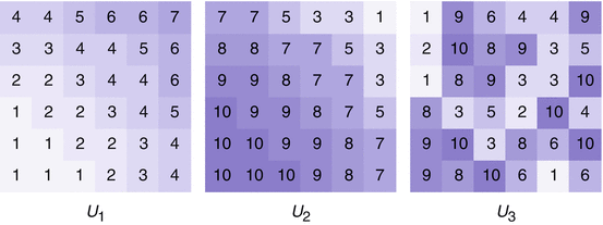
Fig. 3
Images for Examples 2 and 6. Note that there is a dependence between U 1 and U 2: 

Table 1
Comparison of the different pixel-based similarity measures. The images U 1, U 2 are related in a nonlinear way; this is reflected in a correlation ratio of 1. We see that the variance of intensity ratio is not symmetric and not significant to make a statement on a correlation between the images
U 1, U 2 | U 2, U 1 | U 2, U 3 | U 3, U 2 | U 3, U 1 | U 1, U 3 | |
|---|---|---|---|---|---|---|
Correlation coefficient | −0.98 | −0.98 | 0.10 | 0.10 | -0.14 | -0.14 |
Correlation ratio | 1.00 | 1.00 | 0.28 | 0.32 | 0.29 | 0.64 |
Variance of intensity ratio | 1.91 | 2.87 | 2.25 | 1.92 | 3.06 | 0.83 |
Statistical Distance Measures (Density Based)
In general, two images of the same object but of different modalities have a large L p , l p distance. Hence, the idea is to apply statistical tools that consider images as similar if there is some statistical dependence. Statistical similarity measures are able to compare probability density functions. Hence, we first need to relate images to density functions. Therefore, we consider an image as a random variable. The basic terminology of random variables is as follows:
Definition 1.
A continuous random variable is a real-valued function  defined on the sample space Ω S . For a sample x, X(x) is called observation.
 defined on the sample space Ω S . For a sample x, X(x) is called observation.
Remark 1 (Images as Random Variables).
When we consider an image  as a continuous random variable, the sample space is Ω. For a sample x ∈ Ω, the observation u(x) is the intensity of u at x.
 as a continuous random variable, the sample space is Ω. For a sample x ∈ Ω, the observation u(x) is the intensity of u at x.
Regarding the intensity values of an image as an observation of a random process allows us to compare images via their intrinsic probability densities. Since the density cannot be calculated directly, it has to be estimated. This is outlined in section “Density Estimation”. There exists a variety of distance measures for probability densities (see, for instance, [31]). In particular, we review f-divergences in section “Csiszár-Divergences (f-Divergences)” and explain how to use the f-information as an image similarity measure in section “f-Information”.
Density Estimation
This section reviews the problem of density estimation, which is the construction of an estimate of the density function from the observed data.
Definition 2.
Let  be a random variable, that is, a function mapping the (measurable) sample space Ω S of a random process to the real numbers.
 be a random variable, that is, a function mapping the (measurable) sample space Ω S of a random process to the real numbers.
The cumulated probability density function of X is defined by
 The probability density function p is the derivative of P.

The joint cumulated probability density function of two random variables X 1, X 2 is defined by
 The joint probability density function
  satisfies


 satisfies
Remark 2.
When we consider an image  a random variable with sample space Ω, we write p(u)(t) for the probability density function of the image u. For the joint probability of two images u 1 and u 2, we write
  to emphasize, as above, that the images are considered as random variables.
 a random variable with sample space Ω, we write p(u)(t) for the probability density function of the image u. For the joint probability of two images u 1 and u 2, we write
  to emphasize, as above, that the images are considered as random variables.
The terminology of Definition 2 is clarified by the following one-dimensional example:
Example 3.
Let Ω: = [0, 1] and
![$$\displaystyle{\begin{array}{lll} &u: \Omega \ & \rightarrow [0,255]\\ &\ \ \quad x\ &\rightarrow 255x^{2 }.\\ \end{array} }$$](/wp-content/uploads/2016/04/A183156_2_En_4_Chapter_Equx.gif) The cumulated probability density function
The cumulated probability density function
![$$P:\ [0,\ 255] \rightarrow [0,\ 1]$$](/wp-content/uploads/2016/04/A183156_2_En_4_Chapter_Equy.gif) is obtained by integration:
is obtained by integration:
 The probability density function of u is given by the derivative of P, which is
 In image processing, it is common to view the discrete image U(or u N as in (1)) as an approximation of an image u. We aim for the probability density function of u, which is approximated via kernel density estimation using the available information of u, which is U. A kernel histogram is the normalized probability density function according to the discretized image U, where for each pixel a kernel function (see (3)) is superimposed. Kernel functions depend on a parameter, which can be used to control the smoothness of the kernel histogram.
![$$\displaystyle{\begin{array}{lll} &u: \Omega \ & \rightarrow [0,255]\\ &\ \ \quad x\ &\rightarrow 255x^{2 }.\\ \end{array} }$$](/wp-content/uploads/2016/04/A183156_2_En_4_Chapter_Equx.gif)
![$$P:\ [0,\ 255] \rightarrow [0,\ 1]$$](/wp-content/uploads/2016/04/A183156_2_En_4_Chapter_Equy.gif)


We first give a general definition of kernel density estimation:
Definition 3 (Kernel Density Estimation).
Let t 1,  be a sample of M independent observations from a measurable real random variable X with probability density function p. A kernel density approximation at t is given by
![$$\displaystyle{p_{\sigma }(t) = \frac{1} {M}\sum \nolimits _{i=1}^{M}k_{\sigma }(t - t_{ i}),\quad t \in [0,255]}$$](/wp-content/uploads/2016/04/A183156_2_En_4_Chapter_Equab.gif) where
where  is a kernel function with bandwidth
  .
.  is called kernel density approximation with parameter
  .
.
 be a sample of M independent observations from a measurable real random variable X with probability density function p. A kernel density approximation at t is given by
![$$\displaystyle{p_{\sigma }(t) = \frac{1} {M}\sum \nolimits _{i=1}^{M}k_{\sigma }(t - t_{ i}),\quad t \in [0,255]}$$](/wp-content/uploads/2016/04/A183156_2_En_4_Chapter_Equab.gif)
 is a kernel function with bandwidth
  .
.  is called kernel density approximation with parameter
  .
.Let  and
and  be samples of M independent observations from measurable real random variables
  with joint probability density function
  ; then a joint kernel density approximation of
  is given by
 where
where  is a two-dimensional kernel function.
 and
and  be samples of M independent observations from measurable real random variables
  with joint probability density function
  ; then a joint kernel density approximation of
  is given by
 is a two-dimensional kernel function.
Remark 3 (Kernel Density Estimation of an Image, Fig. 4).
Let u be a continuous image, which is identified with a random variable. Moreover, let U be N × N samples of u. In analogy to Definition 3, we denote the kernel density estimation based on the discrete image U, by
 and remark that for u N as in (1)

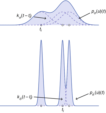


(3)

Fig. 4
Density estimate for different parameters σ
The joint kernel density of two images u 1, u 2 with observations U 1 and U 2 is given by
 where
where  is the two-dimensional kernel function. Moreover, we remark that for
  ,
, 
 In the following, we review particular kernel functions and show that standard histograms are kernel density estimations.

 is the two-dimensional kernel function. Moreover, we remark that for
  ,
, 

Example 4.
Assume that ![$$u_{i}:\ \varOmega \rightarrow [0,\ 255],\ i = 1,\ 2$$](/wp-content/uploads/2016/04/A183156_2_En_4_Chapter_IEq49.gif) are continuous images, with discrete approximations u i, N as in (1):
are continuous images, with discrete approximations u i, N as in (1):
![$$u_{i}:\ \varOmega \rightarrow [0,\ 255],\ i = 1,\ 2$$](/wp-content/uploads/2016/04/A183156_2_En_4_Chapter_IEq49.gif) are continuous images, with discrete approximations u i, N as in (1):
are continuous images, with discrete approximations u i, N as in (1):
We use the joint density kernel , where
  is the normalized Gaussian kernel of variance
  . Then for i = 1, 2, the estimates for the marginal densities are given by
and the joint density approximation reads as follows:


Histograms: Assume that U only takes values in 0, 1, …
Stay updated, free articles. Join our Telegram channel

Full access? Get Clinical Tree


