Methods for Multi-dimensional Visual Data Analysis

can be abstracted from concrete data structures using programming techniques such as generic programming [79]. However, generic algorithms still need to make certain assumptions about the data they operate on. The question remains what these concepts are that describe “data”: what properties should be expected by some algorithm from any kind of data provided for scientific visualization? Moreover, consistency among concepts shared by independent algorithms is also required to achieve interoperability among algorithms and eventually (independently developed) applications. While any particular problem can be addressed by some particular solution, a common concept allows to build a framework instead of just a collection of tools. Tools are what an end user needs to solve a particular problem with a known solution. However, when a problem is not yet clearly defined and a solution unknown, then a framework is required that allows exploration of various approaches and eventually adaption toward a specific direction that does not exist a priori.

The concept of how to lay out data to perform visualization operations in a common framework constitutes a data model for visualization. Many visualization applications are to a greater or lesser extent a collection of tools, even when bundled together within the same software library or binary. Consequently, interoperability between different applications and their corresponding file formats is hard or impossible. Only very few implementations adhere to the vision of a common data model across the various data types for visualization. The idea of a common data model is frequently undervalued or even disregarded as being impossible. However, as D. Butler said, “The proper abstractions for scientific data are known. We just have to use them” [16].

D. Butler was following the mathematical concepts of fiber bundles [16], or more specific, vector bundles [15], to model data. The IBM Data Explorer, one of the earliest visualization applications, now open source and known as “OpenDX (http://www.opendx.org),” implemented this concept successfully [76]. These ideas have been revived and expanded by [7] leading to a hierarchical data structure consisting of a noncyclic graph in seven levels. It can be seen as largely keyword-free, hierarchical version of the OpenDX model, seeking to cast the information and relationships provided in original model into a grouping structure. This data model will be reviewed in the following, together with its mathematical background. Section “Differential Geometry: Manifolds, Tangential Spaces, and Vector Spaces” will review the basic mathematical structures that are used to describe space and time. Section “Topology: Discretized Manifolds” will introduce the mathematical formulation of discretized space. Based on this background, section “Ontological Scheme and Seven-Level Hierarchy” will present a scheme that is able to cover the described mathematical structures.

Differential Geometry: Manifolds, Tangential Spaces, and Vector Spaces

Space and time in physics is modeled via the concept of a differentiable manifold. As scientific visualization deals with data given in space and time, following these concepts is reasonable. In short, a manifold is a topological space that is locally homeomorphic to $\mathbb{R}^{n}$ . However, not all data occurring in scientific visualization are manifolds. The more general case of topological spaces will be discussed in sections “Topology: Discretized Manifolds” and “Topology.”

A vector space over a field F(such as $\mathbb{R}$ ) is a set V together with two binary operations vector addition +: V × V → V and scalar multiplication ∘: F × V → V. The mathematical concept of a vector is defined as an element v ∈ V. A vector space is closed under the operations + and ∘, i.e., for all elements u, v ∈ V and all elements λ ∈ F there is u + v ∈ V and λ ∘ u ∈ V (vector space axioms). The vector space axioms allow computing the differences of vectors and therefore defining the derivative of a vector-valued function $v(s): \mathbb{R} \rightarrow V$ as

$\displaystyle{ \frac{d} {ds}v(s):=\mathop{ \lim }\nolimits _{ds\rightarrow 0}\frac{v(s + ds) - v(s)} {ds} }$

(1)

A manifold in general is not a vector space. However, a differentiable manifold M allows to define a tangential space T _P(M) at each point P which has vector space properties.

Tangential Vectors

In differential geometry, a tangential vector on a manifold M is the operator $\frac{d} {ds}$ that computes the derivative along a curve $q(s): \mathbb{R} \rightarrow M$ for an arbitrary scalar-valued function $f: M \rightarrow \mathbb{R}$ :

$\displaystyle{ \frac{d} {ds}f\Big\vert _{q(s)}:= \frac{df(q(s))} {ds} }$

(2)

Tangential vectors fulfill the vector space axioms and can therefore be expressed as linear combinations of derivatives along the n coordinate functions $x^{\mu }: M \rightarrow \mathbb{R}$ with μ = 0… n − 1, which define a basis of the tangential space T _q(s)(M) on the n-dimensional manifold M at each point q(s) ∈ M:

$\displaystyle{ \frac{d} {ds}f =\sum \nolimits _{ \mu =1}^{n-1}\frac{dx^{\mu }(q(s))} {ds} \frac{\partial } {\partial x^{\mu }}f =:\sum \nolimits _{ \mu =1}^{n-1}\dot{q}^{\mu }\partial _{\mu }f }$

(3)

where {q}^μare the components of the tangential vector $\frac{d} {ds}$ in the chart {x ^μ} and {∂ _μ} are the basis vectors of the tangential space in this chart. In the following text the Einstein sum convention is used, which assumes implicit summation over indices occurring on the same side of an equation. Often tangential vectors are used synonymous with the term “vectors” in computer graphics when a direction vector from point A to point B is meant. A tangential vector on an n-dimensional manifold is represented by n numbers in a chart.

Covectors

The set of operations df: $T(M) \rightarrow \mathbb{R}$ that map tangential vectors v ∈ T(M) to a scalar value v(f) for any function $f: M \rightarrow \mathbb{R}$ defines another vector space which is dual to the tangential vectors. Its elements are called covectors:

$$$\displaystyle{ < df,v >= df(v):= v(f) = v^{\mu }\partial _{\mu }f = v^{\mu }\frac{\partial f} {\partial x^{\mu }} }$$” src=”/wp-content/uploads/2016/04/A183156_2_En_35_Chapter_Equ4.gif”></DIV></DIV><br /> <DIV class=EquationNumber>(4)</DIV></DIV>Covectors fulfill the vector space axioms and can be written as linear combination of covector basis functions <SPAN class=EmphasisTypeItalic>dx</SPAN> <SUP><SPAN class=EmphasisTypeItalic>μ</SPAN> </SUP>:<br /> <DIV id=Equ5 class=Equation><br /> <DIV class=EquationContent><br /> <DIV class=MediaObject><IMG alt=$

(5)

whereby the dual basis vectors fulfill the duality relation

$$$\displaystyle{ < dx^{\nu },\partial _{\mu } >= \left \{\begin{array}{ll} \mu =\nu:&\qquad 1\\ \mu \neq \nu: &\qquad 0\\ \end{array} \right. }$$” src=”/wp-content/uploads/2016/04/A183156_2_En_35_Chapter_Equ6.gif”></DIV></DIV><br /> <DIV class=EquationNumber>(6)</DIV></DIV>The space of covectors is called the cotangential space <SPAN class=EmphasisTypeItalic>T</SPAN> <SUB><SPAN class=EmphasisTypeItalic>P</SPAN> </SUB><SUP>∗</SUP>(<SPAN class=EmphasisTypeItalic>M</SPAN>). A covector on an <SPAN class=EmphasisTypeItalic>n</SPAN>-dimensional manifold is represented by <SPAN class=EmphasisTypeItalic>n</SPAN> numbers in a chart, same as a tangential vector. However, covectors transform inverse to tangential vectors when changing coordinate systems, as is directly obvious from Eq. (<SPAN class=InternalRef><A href=$ 6) in the one-dimensional case: as < dx ⁰, ∂ ₀ > = 1 must be sustained under coordinate transformation, dx ⁰ must shrink by the same amount as ∂ ₀ grows when another coordinate scale is used to represent these vectors. In higher dimensions this is expressed by an inverse transformation matrix.

In Euclidean three-dimensional space, a plane is equivalently described by a “normal vector,” which is orthogonal to the plane. While “normal vectors” are frequently symbolized by an arrow, similar to tangential vectors, they are not the same, rather they are dual to tangential vectors. It is more appropriate to visually symbolize them as a plane. This visual is also supported by (5), which can be interpreted as the total differential of a function f: a covector describes the change of a function f along a direction as specified by a tangential vector $\vec{v}$ . A covector V can thus be visually imagined as a sequence of coplanar (locally flat) planes at distances given by the magnitude of the covector that count the number of planes which are crossed by a vector $\vec{w}$ . This number is V (w). For instance, for the Cartesian coordinate function x, the covector dx “measures” the “crossing rate” of a vector w in the direction along the coordinate line x; see Figs. 1 and 2. On an n-dimensional manifold a covector is correspondingly symbolized by a (n − 1)-dimensional subspace.

Fig. 1

The (trivial) constant vector field along the z-axis viewed as vector field ∂ _zand as covector field dz. (a) Vector field ∂ _z. (b) Duality relationship among ∂ _zand dz. (c) Co-vector field dz

Fig. 2

The basis vector and covector fields induced by the polar coordinates { $r,\vartheta,\phi$ }. (a) Radial field dr ∂ _r. (b) Azimuthal field dϕ ∂ _ϕview of the equatorial plane (z-axis towards eye). (c) Altitudal field dθ ∂ _θslice along the z-axis

Tensors

A tensor T _n^mof rank n × m is a multi-linear map of n vectors and m covectors to a scalar

$\displaystyle{ T_{n}^{m}: T(M) \times \ldots T(M)_{ n} \times T^{{\ast}}(M) \times \ldots T^{{\ast}}(M)_{ m} \rightarrow \mathbb{R} }$

(7)

Tensors are elements of a vector space themselves and form the tensor algebra. They are represented relative to a coordinate system by a set of k ^n+mnumbers for a k-dimensional manifold. Tensors of rank 2 may be represented using matrix notation. Tensors of type T ₁ ⁰ are equivalent to covectors and called co-variant; in matrix notation (relative to a chart) they correspond to rows. Tensors of type T ₀ ¹ are equivalent to a tangential vector and are called contra-variant, corresponding to columns in matrix notation. The duality relationship between vectors and covectors then corresponds to the matrix multiplication of a 1 × n row with a n × 1 column, yielding a single number

$$$\displaystyle{ < a,b >=< a^{\mu }\partial _{\mu },b_{\mu }dx^{\mu } >\;\equiv \; (a^{0}a^{1}\ldots a^{n})\left (\begin{array}{l} b^{0} \\ b^{1}\\ \ldots \\ b^{n}\\ \end{array} \right ) }$$” src=”/wp-content/uploads/2016/04/A183156_2_En_35_Chapter_Equ8.gif”></DIV></DIV><br /> <DIV class=EquationNumber>(8)</DIV></DIV>By virtue of the duality relationship (<SPAN class=InternalRef><A href=$ 6), the contraction of lower and upper indices is defined as the interior product $\iota$ of tensors, which reduces the dimensionality of the tensor:

$\displaystyle{ \iota: T_{n}^{m} \times T_{ k}^{l} \rightarrow T_{ n-1}^{m-k}: u,v\mapsto \iota _{ u}v }$

(9)

The interior product can be understood (visually) as a generalization of some “projection” of a tensor onto another one.

Of special importance are symmetric tensors of rank two g ∈ T ₂ ⁰ with $g: T(M) \times T(M) \rightarrow \mathbb{R}: u,v\mapsto g(u,v),g(u,v) = g(v,u)$ , as they can be used to define a metric or inner product on the tangential vectors. Its inverse, defined by operating on the covectors, is called the co-metric. A metric, same as the co-metric, is represented as a symmetric n × n matrix in a chart for an n-dimensional manifold.

Given a metric tensor, one can define equivalence relationships between tangential vectors and covectors, which allow to map one into each other. These maps are called the “musical isomorphisms,” ♭ and ♯, as they raise or lower an index in the coordinate representation:

$\displaystyle\begin{array}{rcl} \flat: \quad T(M) \rightarrow T^{{\ast}}(M): \quad v^{\mu }\partial _{\mu }\mapsto v^{\mu }g_{\mu \nu }dx^{\nu }& &{}\end{array}$

(10)

$\displaystyle\begin{array}{rcl} \sharp: \quad T^{{\ast}}(M) \rightarrow T(M): \quad V _{\mu }dx^{\mu }\mapsto V _{\mu }g^{\mu \nu }\partial _{\nu }& &{}\end{array}$

(11)

As an example application, the “gradient” of a scalar function is given by ∇f = ♯d f using this notation. In Euclidean space, the metric is represented by the identity matrix and the components of vectors are identical to the components of covectors. As computer graphics usually is considered in Euclidean space, this justifies the usual negligence of distinction among vectors and covectors; consequently graphics software only knows about one type of vectors which is uniquely identified by its number of components. However, when dealing with coordinate transformations or curvilinear mesh types, distinguishing between tangential vectors and covectors is unavoidable. Treating them both as the same type within a computer program leads to confusions and is not safe.

Exterior Product

The exterior product $\wedge: V \times V \rightarrow \varLambda (V )$ is an algebraic construction generating vector space elements of higher dimensions from elements of a vector space V. The new vector space is denoted Λ(V ). It is alternating, fulfilling the property $v \wedge u = -u \wedge v\ \forall u,v \in V$ (which results in $v \wedge v = 0\ \forall v \in V$ ). The exterior product defines an algebra on its elements, the exterior algebra (or Grassmann algebra). It is a sub-algebra of the tensor algebra consisting of the antisymmetric tensors. The exterior algebra is defined intrinsically by the vector space and does not require a metric. For a given n – dimensional vector space V, there can at most be nth power of an exterior product, consisting of n different basis vectors. The (n + 1)th power must vanish, because at least one basis vector would occur twice, and there is exactly one basis vector in Λ ⁿ(V ).

Elements v ∈ Λ ^k(V ) are called k-vectors, whereby two-vectors are also called bi-vectors and three-vectors tri-vectors. The number of components of a k-vector of an n-dimensional vector space is given by the binomial coefficient {n}{k}. For n = 2 there are two one-vectors and one bi-vector, for n = 3 there are three one-vectors, three bi-vectors, and one tri-vector. These relationships are depicted by the Pascal’s triangle, with the row representing the dimensionality of the underlying base space and the column the vector type:

$\displaystyle{ \begin{array}{*{20}c} & & & &1& & & & \\ &&&1&&1&&& \\ & &1& &2& &1& & \\ &1&&3&&3&&1& \\ 1& &4& &6& &4& &1\\ \end{array} }$

(12)

As can be easily read off, for a four-dimensional vector space, there will be four one-vectors, six bi-vectors, four tri-vectors, and one four-vector. The n-vector of an n-dimensional vector space is also called a pseudoscalar, the (n − 1) vector a pseudo-vector.

Visualizing Exterior Products

An exterior algebra is defined on both the tangential vectors and covectors on a manifold. A bi-vector v formed from tangential vectors is written in chart as

$\displaystyle{ v = v^{\mu \nu }\partial _{\mu } \wedge \partial _{\nu } }$

(13)

and a bi-covector U formed from covectors is written in chart as

$\displaystyle{ U = U_{\mu \nu }dx^{\mu } \wedge dx^{\nu } }$

(14)

They both have {n}{2} independent components, due to $v^{\mu \nu } = -v^{\nu \mu }$ and $U_{\mu \nu } = -U_{\nu \mu }$ (three components in 3D, six components in 4D). A bi-tangential vector (13) can be understood visually as an (oriented, i.e., signed) plane that is spun by the two defining tangential vectors, independently of the dimensionality of the underlying base space. A bi-covector (14) corresponds to the subspace of an n-dimensional hyperspace where a plane is “cut out.” In three dimensions these visualizations overlap: both a bi-tangential vector and a covector correspond to a plane, and both a tangential vector and a bi-covector correspond to one-dimensional direction (“arrow”). In four dimensions, these visuals are more distinct but still overlap: a covector corresponds to a three-dimensional volume, but a bi-tangential vector is represented by a plane same as a bi-covector, since cutting out a 2D plane from four-dimensional space yields a 2D plane again. Only in higher dimensions these symbolic representations become unique. However, both a co-vector and a pseudo-vector will always correspond to (i.e., appear as) an (n − 1)-dimensional hyperspace.

$\displaystyle{ V _{\mu }dx^{\mu }\Longleftrightarrow v_{\alpha _{0}\alpha _{1}\ldots \alpha _{n-1}}\partial _{\alpha _{0}} \wedge \partial _{\alpha _{1}} \wedge \ldots \partial _{\alpha _{n-1}} }$

(15)

$\displaystyle{ v^{\mu }\partial _{\mu }\Longleftrightarrow V _{\alpha _{0}\alpha _{1}\ldots \alpha _{n-1}}dx^{\alpha _{0}} \wedge dx^{\alpha _{1}} \wedge \ldots dx^{\alpha _{n-1}} }$

(16)

A tangential vector – lhs of (16) – can be understood as one specific direction. Equivalently, it can be seen as “cutting off” all but one (n − 1)-dimensional hyperspaces from the full n-dimensional space. This equivalence is expressed via the interior product of a tangential vector v with a pseudo-co-scalar Ω yielding a pseudo-covector V (17). Similarly, the interior product of a pseudo-vector with a pseudo-co-scalar yields a tangential vector (17):

$\displaystyle{ \iota _{\varOmega }: T(M) \rightarrow (T^{{\ast}})^{(n-1)}(M): V \mapsto \iota _{\varOmega }v }$

(17)

$\displaystyle{ \iota _{\varOmega }: T^{(n-1)}(M) \rightarrow T^{{\ast}}(M): V \mapsto \iota _{\varOmega }v }$

(18)

Pseudoscalars and pseudo-co-scalars will always be scalar multiples of the basis vectors $\partial _{\alpha 0} \wedge \partial _{\alpha 1} \wedge \ldots \partial _{\alpha n}$ and $dx_{0}^{\alpha } \wedge dx_{1}^{\alpha } \wedge \ldots dx_{n}^{\alpha }$ . However, when inversing a coordinate x ^μ → −x ^μ, they flip sign, whereas a “true” scalar does not. An example known from Euclidean vector algebra is the allegedly scalar value constructed from the dot and cross product of three vectors $V (u,v,w) = u \cdot (v \times w)$ which is the negative of when its arguments are flipped:

$\displaystyle{ V (u,v,w) = -V (-u,-v,-w) = -u \cdot (-v \times -w) }$

(19)

which is actually more obvious when (19) is written as exterior product:

$\displaystyle{ V (u,v,w) = u \wedge v \wedge w = V \partial _{0} \wedge \partial _{1} \wedge \partial _{2} }$

(20)

The result (20) actually describes the multiple of a volume element span by the basis tangential vectors ∂ _μ– any volume must be a scalar multiple of this basis volume element but can flip sign if another convention on the basis vectors is used. This convention depends on the choice of a right-handed versus left-handed coordinate system and is expressed by the orientation tensor $\varOmega = \pm \partial _{0} \wedge \partial _{1} \wedge \partial _{2}$ . In computer graphics, both left-handed and right-handed coordinate systems occur, which may lead to lots of confusions.

By combining (18) and (11) – requiring a metric – we get a map from pseudo-vectors to vectors and reverse. This map is known as the Hodge star operator “*”:

$\displaystyle{ _{{\ast}}: T^{(n-1)}(M) \rightarrow T(M): V \vdash \rightarrow \sharp \iota _{ \Omega }V }$

(21)

The same operation can be applied to the covectors accordingly and generalized to all vector elements of the exterior algebra on a vector space, establishing a correspondence between k – vectors and n – k-vectors. The Hodge star operator allows to identify vectors and pseudo-vectors, similar to how a metric allows to identify vectors and covectors. The Hodge star operator requires a metric and an orientation Ω.

A prominent application in physics using the hodge star operator are the Maxwell equations, which, when written based on the four-dimensional potential $A = V _{0}dx^{0} + A_{k}dx^{k}$ (V ₀ the electrostatic, A _kthe magnetic vector potential), take the form

$\displaystyle{ d_{{\ast}}dA = J }$

(22)

with J the electric current and magnetic flow, which is zero in vacuum. The combination d * d is equivalent to the Laplace operator “ □ ,” which indicates that (22) describes electromagnetic waves in vacuum.

Geometric Algebra

Geometric Algebra is motivated by the intention to find a closed algebra on a vector space with respect to multiplication, which includes existence of an inverse operation. There is no concept of dividing vectors in “standard” vector algebra. Neither the inner or outer product has provided vectors of the same dimensionality as their arguments, so they do not provide a closed algebra on the vector space.

Geometric Algebra postulates a product on elements of a vector space u, v, w $\in \mathcal{V}$ that is associative (uv)w = u(vw), left distributive $$u(v + w) = uv + uw$$

, and right distributive ( $$u + v)w = uw + vw$$

and reduces to the inner product as defined by the metric v ² = g(v, v). It can be shown that the sum of the outer product and the inner product fulfill these requirements; this defines the geometric product as the sum of both:

$\displaystyle{ uv:= u \wedge v + u \cdot v }$

(23)

Since $u \wedge v$ and $u \cdot v$ are of different dimensionalities ({n} {{2} and {n} {{0}, respectively), the result must be in a higher-dimensional vector space of dimensionality {n} {{2} + {n} {{0}. This space is formed by the linear combination of k-vectors; its elements are called multivectors. Its dimensionality is $\sum \nolimits _{k=0}^{n-1}\left (\begin{array}{l} n\\ k\\ \end{array} \right ) \equiv 2^{n}$ .

For instance, in two dimensions, the dimension of the space of multivectors is 2² = 4. A multivector V, constructed from tangential vectors on a two-dimensional manifold, is written as

$\displaystyle{ V = V ^{0} + V ^{1}\partial _{ 0} + V ^{2}\partial _{ 1} + V ^{3}\partial _{ 0} \wedge \partial _{1} }$

(24)

with V ^μthe four components of the multivector in a chart. For a three-dimensional manifold, a multivector on its tangential space has 2³ = 8 components and is written as

$\displaystyle{ \begin{array}{ll} V =&V ^{0}+ \\ &V ^{1}\partial _{0} + V ^{2}\partial _{1} + V ^{2}\partial _{2}+ \\ &V ^{4}\partial _{0} \wedge \partial _{1} + V ^{5}\partial _{1} \wedge \partial _{2} + V ^{6}\partial _{2} \wedge \partial _{0}+ \\ &V ^{7}\partial _{0} \wedge \partial _{1} \wedge \partial _{2}\\ \end{array} }$

(25)

with V ^μthe eight components of the multivector in a chart. The components of a multivector have a direct visual interpretation, which is one of the key features of Geometric Algebra. In 3D, a multivector is the sum of a scalar value, three directions, three planes, and one volume. These basis elements span the entire space of multivectors. Geometric Algebra provides intrinsic graphical insight to the algebraic operations. Its application for computer graphics will be discussed in Sect. 4.

Vector and Fiber Bundles

The concept of a fiber bundle data model is inspired by its mathematical correspondence. In short, a fiber bundle is a topological space that looks locally like a product space B × F of a base space B and a fiber space F.

The fibers of a function f: X → Y are the pre-images or inverse images of the points y ∈ Y, i.e., the sets of all elements x ∈ X with f(x) = y:

$\displaystyle{f^{-1}(y) =\{ x \in X\vert f(x) = y\}}$

is a fiber of f (at the point y). A fiber can also be the empty set. The union set of all fibers of a function is called the total space. The definition of a fiber bundle makes use of a projection mappr ₁, which is a function that maps each element of a product space to the element of the first space:

$\displaystyle\begin{array}{rcl} pr_{1}: X \times Y \quad & \rightarrow & \quad X {}\\ (x,y)\quad & \longmapsto & \quad x {}\\ \end{array}$

Let E, B be topological spaces and f: E → B a continuous map. (E, B, f) is called a (fiber) bundle if there exists a space F such that the union of fibers of a neighborhood U _b ⊂ B of each point b ∈ B is homeomorphic to U _b× F such that the projection pr ₁ of U _b× F is U _bagain:

$\displaystyle{\begin{array}{l} (E,B,f: E \rightarrow B)\;\mbox{ bundle}\Longleftrightarrow\exists F: \forall b \in B: \exists U_{b}: f^{-1}(U_{b})\mathop{\simeq }\limits ^{\hom }U_{b} \times F \\ \quad \quad \quad \quad \quad \quad \quad \quad \quad \quad \quad \quad \mbox{ and}\quad pr_{1}(U_{b} \times F) = U_{b}\\ \end{array} }$

E is called the total space E, B is called the base space, and f: E → B the projection map. The space F is called the fiber type of the bundle or simply the fiber of the bundle. In other words, the total space can be written locally as a product space of the base space with some space F. The notation $\mathcal{F}(B) = (E,B,f)$ will be used to denote a fiber bundle over the base space B. It is also said that the space F fibers over the base space B.

An important case is the tangent bundle, which is the union of all tangent spaces T _p(M) on a manifold M together with the manifold $\mathcal{T} (M):= \{(p,v): p \in M,v \in T_{p}(M)\}$ . Every differentiable manifold possesses a tangent bundle $\mathcal{T} (M)$ . The dimension of $\mathcal{T} (M)$ is twice the dimension of the underlying manifold M, its elements are points plus tangential vectors. T _p(M) is the fiber of the tangent bundle over the point p.

If a fiber bundle over a space B with fiber F can be written as B × F globally, then it is called a trivial bundle (B × F, B, pr ₁). In scientific visualization, usually only trivial bundles occur. A well-known example for a nontrivial fiber bundle is the Möbius strip.

Topology: Discretized Manifolds

For computational purposes, a topological space is modeled by a finite set of points. Such a set of points intrinsically carries a discrete topology by itself, but one usually considers embeddings in a space that is homeomorphic to Euclidean space to define various structures describing their spatial relationships.

A subset c ⊂ X of a Hausdorff space X is a k-cell if it is homeomorphic to an open k-dimensional ball in $\mathbb{R}^{n}$ . The dimension of the cell is k. Zero-cells are called vertices, one-cells are edges, two-cells are faces or polygons, and three-cells are polyhedra – see also section “Chains.” An n-cell within an n-dimensional space is just called a “cell.” (n − 1)-cells are sometimes called “facets” and (n − 2)-cells are known as “ridges.” For k-cells of arbitrary dimension, incidence and adjacency relationships are defined as follows: two cells c ₁, c ₂ are incident if c ₁ ⊆ ∂ c ₂, where ∂ c ₂ denotes the border of the cell c ₂. Two cells of the same dimension can never be incident because dim(c ₁) ≠ dim(c ₂) for two incident cells c ₁, c ₂. c ₁ is a side of c ₂ if dim(c ₁) < dim(c ₂), which may be written as c ₁ < c ₂. The special case ${\mathrm{dim}}(c_{1}) =\mathrm{ dim}(c_{2}) - 1$ may be denoted by c ₁ ≺ c ₂. Two k -cells c ₁, c ₂ with k > 0 are called adjacent if they have a common side, i.e.,

$\displaystyle{\mbox{ cell}\;c_{1},c_{2}\quad \mathbf{adjacent}\Longleftrightarrow\exists \quad \mbox{ cell}\;f:\; f < c_{1},f < c_{2}}$

For k = 0, two zero-cells (i.e., vertices) v ₁, v ₂ are said to be adjacent if there exists a one-cell (edge) e which contains both, i.e., v ₁ < e and v ₂ < e. Incidence relationships form an incidence graph. A path within an incidence graph is a cell tuple: a cell-tuple $\mathcal{C}$ within an n-dimensional Hausdorff space is an ordered sequence of k-cells $(c_{n},c_{n-1},\ldots,c_{1},c_{0})$ of decreasing dimensions such that $\forall 0 < i \leq n: c_{i-1} \prec c_{i}$ . These relationships allow to determine topological neighborhoods: adjacent cells are called neighbors. The set of all k + 1 cells which are incident to a k-cell forms a neighborhood of the k-cell. The cells of a Hausdorff space X constitute a topological base, leading to the following definition: a (“closure-finite, weak-topology”) CW-complex $\mathcal{C}$ , also called a decomposition of a Hausdorff space X, is a hierarchical system of spaces $X^{(-1)} \subseteq X^{(0)} \subseteq X^{(1)} \subseteq \ldots \subseteq X^{(n)}$ , constructed by pairwise disjoint open cells c ⊂ X with the Hausdorff topology $\cup ^{c\in \mathcal{C}^{\mathcal{C}} }$ , such that X ⁽ⁿ⁾ is obtained from X ⁽ⁿ⁻¹⁾ by attaching adjacent n-cells to each (n − 1)-cell and $X^{(-1)} =\emptyset$ . The respective subspaces X ⁽ⁿ⁾ are called the n-skeletons of X. A CW complex can be understood as a set of cells which are glued together at their subcells. It generalizes the concept of a graph by adding cells of dimension greater than 1.

Up to now, the definition of a cell was just based on a homeomorphism of the underlying space X and $\mathbb{R}^{n}$ . Note that a cell does not need to be “straight,” such that, e.g., a two-cell may be constructed from a single vertex and an edge connecting the vertex to itself, as, e.g., illustrated by J. Hart [34]. Alternative approaches toward the definition of cells are more restrictively based on isometry to Euclidean space, defining the notion of “convexity” first. However, it is recommendable to avoid the assumption of Euclidean space and treating the topological properties of a mesh purely based on its combinatorial relationships.

Ontological Scheme and Seven-Level Hierarchy

The concept of the fiber bundle data model builds on the paradigm that numerical data sets occurring for scientific visualization can be formulated as trivial fiber bundles (see section “Vector and Fiber Bundles”). Hence, data sets may be distinguished by their properties in the base space and the fiber space. At each point of the – discretized – base space, there are some data in the fiber space attached. Basically a fiber bundle is a set of points with neighborhood information attached to each of them. An n-dimensional array is a very simple case of a fiber bundle with neighborhood information given implicitly.

The structure of the base space is described as a CW complex, which categorizes the topological structure of an n-dimensional base space by a sequence of k-dimensional skeletons, with 0 < k < n. These skeletons carry certain properties of the data set: the zero-skeleton describes vertices, the one-skeleton refers to edges, two-skeleton to the faces, etc., of some mesh (a triangulation of the base space). Structured grids are triangulations with implicitly given topological properties. For instance, a regular n-dimensional grid is one where each point has 2ⁿneighbors.

The structure of the fiber space is (usually) not discrete and given by the properties of the geometrical object residing there, such as a scalar, vector, covector, and tensor. Same as the base space, the fiber space has a specific dimensionality, though the dimensionality of the base space and fiber space is independent. Figure 3 demonstrates example images from scientific visualization classified via their fiber bundle structure. If the fiber space has vector space properties, then the fiber bundle is a vector bundle and vector operations can be performed on the fiber space, such as addition, multiplication, and derivation.

Fig. 3

Fiber bundle classification scheme for visualization methods:dimensionality of the base space (involving the k-skeleton of the discretized manifold) and dimensionality of the fiber space (involving the number of field quantities per element, zero referring to display of the mere topological structure). (a) Zero-cells, 0D. (b) Zero-cells, 1D. (c) Zero-cells, 3D. (d) Zero-cells, 6D. (e) One-cells, 0D. (f) One-cells, 1D. (g) One-cells, 3D. (h) One-cells, 6D. (i) Two-cells, 0D. (j) Two-cells, 1D. (k) Two-cells, 3D. (l) Two-cells, 6D. (m) Three-cells, 0D. (n) Three-cells, 1D. (o) Three-cells, 3D. (p) Three-cells, 6D

The distinction between base space and fiber space is not common use in computer graphics, where topological properties (base space) are frequently intermixed with geometrical properties (coordinate representations). Operations in the fiber space can, however, be formulated independently from the base space, which leads to a more reusable design of software components. Coordinate information, formally part of the base space, can as well be considered as fiber, leading to further generalization. The data sets describing a fiber are ideally stored as contiguous arrays in memory or disk, which allows for optimized array and vector operations. Such a storage layout turns out to be particularly useful for communicating data with the GPU using vertex buffer objects: the base space is given by vertex arrays (e.g., OpenGL glVertexPointer), and fibers are attribute arrays (e.g., OpenGL glVertexAttribPointer), in the notation of computer graphics. While the process of hardware rendering in its early times had been based on procedural descriptions (cached in display lists), vertex buffer objects are much faster in state-of-the-art technology. Efficient rendering routines are thus implemented as maps from fiber bundles in RAM to fiber bundles in GPU memory (eventually equipped with a GPU shader program).

A complex data structure (such as some color-coded time-dependent geometry) will be built from many data arrays. The main question that needs to be answered by a data model is how to assign a semantic meaning to each of these data arrays – what do the numerical values actually mean? It is always possible to introduce a set of keywords with semantics attached to them. In addition, the introduction of keywords also reduces the number of possible identifiers available for user-specific purpose. This problem is also known as “name space pollution”. The approach followed in the data model presented in [7] is to avoid use of keywords as much as possible. Instead, it assigns the semantics of an element of the data structure into the placement of this element. The objective is to describe all data types that occur in an algorithm (including file reader and rendering routines) within this model. It is formulated as a graph of up to seven levels (two of them optional). Each level represents a certain property of the entire data set, the Bundle. These levels are called:

Slice

Grid

Skeleton

Representation

Field

(Fragment)

(Compound Elements)

Actual data arrays are stored only below the “Field” level. Given one hierarchy level, the next one is accessed via some identifier. The type of this identifier differs for each level: numerical values within a Skeleton level are grouped into Representation objects, which hold all information that is relative to a certain “representer.” Such a representer may be a coordinate object that, for instance, refers to some Cartesian or polar chart, or it may well be another Skeleton object, either within the same Grid object or even within another one. An actual data set is described through the existence of entries in each level. Only two of these hierarchy levels are exposed to the end user; these are the Grid and Field levels. Their corresponding textual identifiers are arbitrary names specified by the user.

Hierarchy object	Identifier type	Identifier semantic
Bundle	Floating point number	Time value
Slice	String	Grid name
Grid	Integer set	Topological properties
Skeleton	Reference	Relationship map
Representation	String	Field name
Field	Multidimensional index	Array index

A Grid is subset of data within the Bundle that refers to a specific geometrical entity. A Grid might be a mesh carrying data such as a triangular surface, a data cube, a set of data blocks from a parallel computation, or many other data types. A Field is the collection of data sets given as numbers on a specific topological component of a Grid, for instance, floating point values describing pressure or temperature on a Grid’s vertices. All other levels of the data model describe the properties of the Bundle as construction blocks. The usage of these construction blocks constitutes a certain language to describe data sets. A Slice is identified by a single floating point number representing time (generalization to arbitrary-dimensional parameter spaces is possible). A Skeleton is identified by its dimensionality, index depth (relationship to the vertices of a Grid), and refinement level. This will be explained in more detail in section “Topological Skeletons.” The scheme also extends to cases beyond the purely mathematical basis to also cover data sets that occur in praxis, which is described in section “Non-topological representations.” A representation is identified via some reference object, which may be some coordinate system or another Skeleton. The lowest levels of fragments and compounds describe the internal memory layout of a Field data set and are optional; some examples are described in [8, 9].

Field Properties

A specific Field identifier may occur in multiple locations. All these locations together define the properties of a field. The following four properties are expressible in the data model:

Hierarchical ordering: For a certain point in space, there exist multiple data values, one for each refinement level. This property describes the topological structure of the base space.

Multiple coordinate systems: One spatial point may have multiple data representations relating to different coordinate systems. This property describes the geometrical structure of the base space.

Fragmentation: Data may stem from multiple sources, such as a distributed multiprocess simulation. The field then consists of multiple data blocks, each of them covering a subdomain of the field’s base space. Such field fragments may also overlap, known as “ghost zones.”

Separated Compounds: A compound data type, such as a vector or tensor, may be stored in different data layouts since applications have their own preferences. An array of tensors may also be stored as a tensor of arrays, e.g., XYZXYZXYZXYZ as XXXXYYYYZZZZ. This property describes the internal structure of the fiber space.

All of these properties are optional. In the most simple case, a field is just represented by an array of native data types; however, in the most general case (which the visualization algorithm must always support), the data are distributed over several such property elements and built from many arrays. With respect to quick transfer to the GPU, only the ability to handle multiple arrays per data set is of relevance.

Figure 4 illustrates the organization of the last four levels of the data model. These consist of Skeleton and Representation objects with optional fragmentation and compound levels. The ordering of these levels is done merely based on their semantic importance, with the uppermost level (1) embracing multiple resolutions of the spatial domain being the most visible one to the end user. Each of these resolution levels may come with different topological properties, but all arrays within the same resolution are required to be topologically compatible (i.e., share the same number of points). There might still be multiple coordinate representations required for each resolution, which constitutes the second hierarchy level (2) of multiple coordinate patches. Data per patch may well be distributed over various fragments (3), which is considered an internal structure of each patch, due to parallelization or numerical issues, but not fundamental to the physical setup. Last but not least, fields of multiple components such as vector or tensor fields may be separated into distinct arrays themselves [7]. This property, merely a performance issue of in-memory data representation, is not what the end user usually does not want to be bothered with and is thus set as the lowest level in among these four entries.

Fig. 4

Hierarchical structure of the data layout of the concept of a field in computer memory: (1) organization by multiple resolutions for same spatial domain; (2) multiple coordinate systems covering different spatial domains (arbitrary overlap possible); (3) fragmentation of fields into blocks (recombination from parallel data sources); and (4) layout of compound fields as components for performance reasons, indicated as S (scalar field), {x, y, z} for vector fields, and {xx, xy, yy, yz, zz, zx} for tensor fields

Fig. 5

The five-level organization scheme used for atmospheric data (MM5 model data) and surge data (ADCIRC simulation model), built upon common topological property descriptions with additional fields (From Venkataraman et al. [81])

Topological Skeletons

The Skeleton level of the fiber bundle hierarchy describes a certain topological property. This can be the vertices, the cells, the edges, etc. Its primary purpose is to describe the skeletons of a CW complex, but they may also be used to specify mesh refinement levels and agglomerations of certain elements. All data fields that are stored within a Skeleton level provide the same number of elements. In other words they share their index space (a data space in HDF5 terminology). Each Topology object within a Grid object is uniquely identified via a set of integers, which are the dimension (e.g., the dimension of a k-cell), index depth (how many dereferences are required to access coordinate information in the underlying manifold), and refinement level (a multidimensional index, in general). Vertices – index depth 0 – of a topological space of dimension n define a Skeleton of type (n, 0). Edges are one-dimensional sets of vertex indices; therefore, their index depth is 1 and their Skeleton type is (1,1). Faces are two-dimensional sets of vertex indices, hence Skeleton type (2, 1). Cells – such as a tetrahedron or hexahedra – are described by a Skeleton type (3, 1). All the Skeleton objects of index depth 1 build the k-skeletons of a manifold’s triangulation.

Higher index depths describe sets of k-cells. For instance, a set of edges describes a line – a path along vertices in a Grid. Such a collection of edges will fit into a Skeleton of dimension 1 and depth 2, i.e., type (1, 2). It is a one-dimensional object of indices that refer to edges that refer to vertices.

Non-topological Representations

Polynomial coordinates, information on field fragments, histograms, and color maps can be formulated in the fiber bundle model as well. These quantities are no longer direct correspondences of the mathematical background, but they may still be cast into the given context.

Coordinates may be given procedurally, such as via some polynomial expression. The data for such expressions may be stored in a Skeleton of negative index depth – as these data are required to compute the vertex coordinates and more fundamental than these in this case.

A fragment of a Field given on vertices – the (n, 0)-Skeleton of a Grid – defines an n-dimensional subset of the Grid, defined by the hull of the vertices corresponding to the fragments. These may be expressed as a (n, 2)-Skeleton, where the Field object named “Positions” (represented relative to the vertices) refers to the (global) vertex indices of the respective fragments. The representation in coordinates corresponds to its range, known as the bounding box. Similarly, a field given on the vertices will correspond to the field’s numerical minimum/maximum range within this fragment.

A histogram is the representation of a field’s vertex complex in a “chart” describing the required discretization, depending on the min/max range and a number count. A color map (transfer function) can be interpreted as a chart object itself. It has no intrinsically geometrical meaning, but provides means to transform some data. For instance, some scalar value will be transformed to some RGB triple using some color map. A scalar field represented in a certain color map is therefore of type RGB values and could be stored as an array of RGB values for each vertex. In practice, this will not be done since such transformation is performed in real time by modern graphics hardware. However, this interpretation of a color map as a chart object tells how color maps may be stored in the fiber bundle data model.

3 Differential Forms and Topology

This section not only introduces the concepts of differential forms and their discrete counterparts but also illustrates that similar concepts are applied in several separate areas of scientific visualization. Since the available resources are discrete and finite, concepts mirroring these characteristics have to be applied to visualize complex data sets. The most distinguished algebraic structure is described by exterior algebra (or Grassmann algebra, see also section “Exterior Product”), which comes with two operations, the exterior product (or wedge product) and the exterior derivative.

Differential Forms

Manifolds can be seen as a precursor to model physical quantities of space. Charts on a manifold provide coordinates, which allows using concepts which are already well established. Furthermore, they are crucial for the field of visualization, as they are key components to obtain depictable expressions of abstract entities. Tangential vectors were already introduced in section “Tangential Vectors” as derivatives along a curve. Then a one-form α is defined as a linear mapping which assigns a value to each tangential vector v from the tangent space T _P(M), i.e., $\alpha: T_{P}(M) \rightarrow \mathbb{R}$ . They are commonly called co-variant vectors, covectors (see section “Tangential Vectors”), or Pfaff-forms. The set of one-forms generates the dual vector space or cotangential space T _p^∗(M). It is important to highlight that the tangent vectors v ∈ T _P(M) are not contained in the manifold itself, so the differential forms also generate an additional space over P ∈ M. In the following, these one-forms are generalized to (alternating) differential forms.

An alternative point of view treats a tangential vector $$v$$

as a linear mapping which assigns a scalar to each one-form α by $$$<\alpha,v >\in \mathbb{R}$$” src=”/wp-content/uploads/2016/04/A183156_2_En_35_Chapter_IEq49.gif”></SPAN>. By omitting one of the arguments of the obtained mappings, < <SPAN class=EmphasisTypeItalic>α</SPAN>, . > or <SPAN class=EmphasisTypeItalic>α</SPAN>(<SPAN class=EmphasisTypeItalic>v</SPAN>) and < ., <SPAN class=EmphasisTypeItalic>v</SPAN> > or <SPAN class=EmphasisTypeItalic>v</SPAN>(<SPAN class=EmphasisTypeItalic>α</SPAN>), linear objects are defined. Multi-linear mappings depending on multiple vectors or covectors appear as an extension of this concept and are commonly called tensors<br /> <DIV id=Equ27 class=Equation><br /> <DIV class=EquationContent><br /> <DIV class=MediaObject><IMG alt=$

(26)

where n and m are natural numbers and T ⁿand T ^∗mrepresent the n and m powered Cartesian product of the tangential space or the dual vector space (cotangential space). A tensor γ is called an (n, m)-tensor which assigns a scalar value to a set of m covectors and n vectors. All tensors of a fixed type (n, m) generate a tensor space attached at the point P ∈ M. The union of all tensor spaces at the points P ∈ M is called a tensor bundle. The tangential and cotangential bundles are specialized cases for (1, 0) and (0, 1) tensor bundles, respectively. Fully antisymmetric tensors of type (0, m) may be identified with differential forms of degree m. For m > dim(M), where dim(M) represents the dimension of the manifold, differential forms vanish.

The exterior derivative or Cartan derivative of differential forms generates a p + 1-form df from a p-form f and conforms to the following requirements:

Compatibility with the wedge product (product rule): $d(\alpha \wedge \beta ) = d\alpha \wedge \beta +(-1)^{m}\alpha \wedge d\beta$

Nilpotency of the operation d, d ∘ d = 0, depicted in Fig. 11

Linearity

A subset of one-forms is obtained as a differential df of zero-forms (functions) f at P and are called exact differential forms. For an n-dimensional manifold M, a one-form can be depicted by drawing (n − 1)-dimensional surfaces, e.g., for the three-dimensional space, Fig. 6 depicts a possible graphical representation of a one-form attached to M. This depiction also enables a graphical representation on how to integrate differential forms, where only the number of surfaces which are intersected by the integration domain has to be counted:

$$$\displaystyle{ < df,v >= df(v) =\alpha (v) }$$” src=”/wp-content/uploads/2016/04/A183156_2_En_35_Chapter_Equ28.gif”></DIV></DIV><br /> <DIV class=EquationNumber>(27)</DIV></DIV></DIV></DIV><br /> <DIV class=ClearBoth> </DIV></DIV></DIV><br /> <DIV id=Fig6 class=Figure><br /> <DIV class=MediaObject><IMG alt=A183156_2_En_35_Fig6_HTML.jpg src=$

Fig. 6

Possible graphical representation of the topological structure of one-forms in three dimensions. Note that the graphical display of differential forms varies in different dimension and does not depend on the selected basis elements

A consequence of being exact includes the closeness property d α = 0. Furthermore, the integral $\int _{C_{p}}df$ with C _prepresenting an integration domain, e.g., an interval x ₁ and x ₂, results in the same value f(x ₂) − f(x ₁). In the general case, a p-form is not always the exterior derivative of a p-one-form; therefore, the integration of p-forms is not independent of the integration domain. An example is given by the exterior derivative of a p-form β resulting in a p + 1-form γ = d β. The structure of such a generated differential form can be depicted by a tube-like structure such as in Fig. 7. While the wedge product of an r-form and an s-form results in an r + s-form, this resulting form is not necessarily representable as a derivative. Figure 7 depicts a two-form which is not constructed by the exterior derivative but instead by $\alpha \wedge \beta$ , where α and β are one-forms. In the general case, a p-form attached on an n-dimensional manifold M is represented by using (n − p)-dimensional surfaces.

Fig. 7

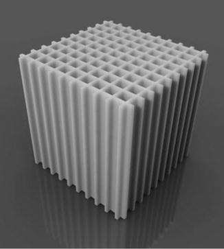
Possible graphical representation of a general two-form generated by $\alpha \wedge \beta$ , where α and β are one-forms. The topologically tube-like structure of the two-forms is enclosed by the depicted planes

By sequentially applying the operation d to (0, m) for 0 ≤ m ≤ dim(M), the de Rham complex is obtained, which enables the investigation of the relation of closed and exact forms. The de Rham complex enables the transition from the continuous differential forms to the discrete counterpart, so-called cochains. The already briefly mentioned topic of integration of differential forms is now mapped onto the integration of these cochains. To complete the description, the notion of chains, also modeled by multivectors (as used in Geometric Algebra, see section “Geometric Algebra” and Sect. 4) or fully antisymmetric (n, 0)-tensors, as description of integration domains is presented, where a chain is a collection of n-cells.

The connection between chains and cochains is investigated in algebraic topology under the name of homology theory, where chains and cochains are collected in additive Abelian groups C _p(M).

Chains

The de Rham complex collects cochains similar to a cell complex aggregating cells as elements of chains. To use these elements, e.g., all edges, in a computational manner, a mapping of the n-cells onto an algebraic structure is needed. An algebraic representation of the assembly of cells, an n-chain, over a cell complex $\mathcal{K}$ and a vector space $\mathcal{V}$ can be written by

$\displaystyle{c_{n} =\sum \nolimits _{ i=1}^{j}w_{ i}\tau _{n}^{i}\quad \tau _{ n}^{i} \in \;\mathcal{K},\;w_{ i} \in \;\mathcal{V}}$

which is closed under reversal of the orientation:

$\displaystyle{\forall \tau _{n}^{i} \in c_{ n}\quad \mbox{ there}\;\mbox{ is} -\tau _{n}^{i} \in c_{ n}}$

The different topological elements are called cells, and the dimensionality is expressed by adding the dimension such as a three-cell for a volume, a two-cell for surface elements, a one-cell for lines, and a zero-cell for vertices. If the coefficients are restricted to { − 1, 0, 1} ∈ $\mathbb{Z}$ , the following classification for elements of a cell complex is obtained:

0: if the cell is not in the complex
1: if the unchanged cell is in the complex
− 1: if the orientation is changed

The so-called boundary operator is a map between sets of chains C _pon a cell complex K. Let us denote the ith p-cell as $\tau _{p}^{i} = k_{0},\ldots k_{p}$ , whereby τ _pⁱ ∈ K. The boundary operator ∂ _pdefines a (p − 1)-chain computed from a p-chain: $\partial _{p}: C_{p}(K) --\rightarrow C_{p-1}(K)$ . The boundary of a cell τ _p^jcan be written as alternating sum over elements of dimension p − 1:

$\displaystyle{ \partial _{p}\tau _{p}^{i} =\sum \nolimits _{ i}(-1)^{i}[k_{ 0},k_{1},\ldots,\tilde{k}_{i},\ldots k_{n}] }$

(28)

where $\tilde{k}_{i}$ indicates that k _iis deleted from the sequence. This map is compatible with the additive and the external multiplicative structure of chains and builds a linear transformation:

$\displaystyle{ C_{p} \rightarrow C_{p-1} }$

(29)

Therefore, the boundary operator is linear

$\displaystyle{ \partial \left (\sum \nolimits _{i}w_{i}\tau _{p}^{i}\right ) =\sum \nolimits _{ i}w_{i}\left (\partial \tau _{p}^{i}\right ) }$

(30)

which means that the boundary operator can be applied separately to each cell of a chain. Using the boundary operator on a sequence of chains of different dimensions results in a chain complex C _∗ = {C _p, ∂ _p} such that the complex property

$\displaystyle{ \partial _{p-1}\partial _{p} = 0 }$

(31)

is given. Homological concepts are visible here for the first time, as homology examines the connectivity between two immediately neighboring dimensions. Figure 8 depicts two examples of one-chains and two-chains and an example of the boundary operator.