Analysis of Diffusion Tensor MRI in Simulated Rat Myocardium

is the estimated mean of the elementary effects and estimates the overall effect of the factor on the output, and $\sigma$ is the standard deviation of the elementary effects and estimates non-linear effects and interactions with other factors. Campolongo et al. [10] introduced a modified version, $\mu ^*$ , which uses absolute values and avoids effects of opposite signs.

The aim of this study is, firstly, to demonstrate a modelling methodology in the heart and to qualitatively assess the similarity of experimental and simulated measurements. Secondly, we aim to determine which parameters related to the cell and tissue geometry of rat myocardium have the greatest influence on DTI measurements. This will inform future studies investigating the effect of cardiac microstructure on DTI results.

2 Methods

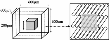
A model of a simplified volume of left ventricular myocardium was created using Smoldyn [11], as shown in Fig. 1. All anatomical and physiological parameters in the model are adopted from the literature, with their ranges reflecting the range of values reported in different publications. Cells are modelled as cuboids with a defined length (L), cross-sectional area (CSA) and aspect ratio of the cross-section (AR, thickness/width). The model consists of layers of cells where each layer is parallel to the epicardium and endocardium, that is, transverse angles (those between the circumferential axis and the projection of the cell’s long axis onto the radial-circumferential plane [16]) are set to $0^{\circ }$ . Cells within each layer are parallel to each other. The spacing of the cells and layers was chosen to give the desired volume fraction (VF) of cells, that is, the proportion of the tissue made up of myocytes. In the central layer, the helix angle (that between the cell’s long axis projected onto a plane parallel to the epicardium, and the radial-circumferential plane [16]) is set to $45^{\circ }$ . The helix angle varies linearly across the voxel at a rate (ANG) based on both typical left ventricular (LV) wall thickness and the range of helix angles found across the myocardium. A single cubic voxel was analysed with sides of 200 ${\upmu \mathrm {m}}$ . To avoid boundary effects, a cube with sides of 600 ${\upmu \mathrm {m}}$ was modelled, with the ‘voxel’ at the centre of this. $4 \times 10^6$ molecules were randomly distributed across the simulation volume. At each time step, each molecule moves in a random direction with a step length normally distributed about a mean which is proportional to the diffusivity (DIF). If the molecule reaches a boundary, it reflects off that boundary. The chosen values for the sensitivity analysis parameters are in Table 1 and are based on values found in the literature [7, 8, 12–16].

Table 1.

Sensitivity analysis parameters, based on [7, 8, 12–16]

Parameter	Abbreviation	Units	Minimum value	Maximum value
Cross-sectional area	CSA	$\mathrm {\mu m^2}$	100	300
Length	L	$\mathrm {\mu m}$	90	150
Aspect ratio (thickness/width)	AR		0.33	1.00
Volume fraction of myocytes	VF		0.75	0.90
Angle range	ANG	$\mathrm {^{\circ }/mm}$	50	100
Diffusivity	DIF	$\mathrm {mm^2/s}$	$0.5 \times \,10^{-3}$	$2.5 \times \,10^{-3}$

Fig. 1.

Model geometry. ‘Voxel’ to be analysed is grey cube at centre of total model volume. Right image shows a typical arrangement of the cells (cuboids) in the central layer, with the grey area indicating the voxel. All layers are parallel to each other.

Custom-written Matlab code was used to calculate the total phase shift, $\varPsi$ , for each molecule from their locations. It is a function of the gradient strength that it experiences over every timestep j, and is calculated as [8]:

$\begin{aligned} \varPsi = \sum _{j=0}^N\varPsi _j = \sum _{j=0}^N\gamma \langle G(t_j),r(t_j) \rangle \delta t \end{aligned}$

(1)

where N is the total number of timesteps,

is the magnetic field gradient at timestep j, and

is the molecule position at timestep j. The MRI signal,

, for all M molecules is then:

$\begin{aligned} \frac{S}{S_0} = \frac{1}{M}\sum _{i=1}^M\cos (\varPsi ) \end{aligned}$

(2)

The DT was calculated, the fibre angle was that between the primary eigenvector and the x-y plane, and the FA and ADC were calculated from [6]:

$\begin{aligned} ADC= \frac{\lambda _1+\lambda _2+\lambda _3}{3} \end{aligned}$

(3)

$\begin{aligned} FA= \sqrt{\frac{3}{2}} \sqrt{\frac{(\lambda _1-\bar{\lambda })^2+(\lambda _2-\bar{\lambda })^2 + (\lambda _3-\bar{\lambda })^2}{\lambda _1^2+\lambda _2^2+\lambda _3^2 }} \end{aligned}$

(4)

where $\lambda _i$ is the i^th eigenvalue and $\bar{\lambda }$ is the mean of the eigenvalues.

Modified Morris method [10] parameters were generated and analysed using the Matlab (Mathworks, USA) code of [17]. A b-value of 1474 $\mathrm {s/mm^2}$ was used (experiment 1 in Table 2), which is similar to the experimental data. The b-value combines the properties of the applied gradient pulse into a single factor. In the idealised free diffusion state for rectangular pulses, this is given by:

$\begin{aligned} b = (G\gamma \delta )^2(\varDelta - \frac{\delta }{3}) \end{aligned}$

(5)

where G is the magnetic field gradient strength, $\delta$ is the diffusion pulse duration, $\varDelta$ is the time between pulse onsets, and $\gamma$ is the gyromagnetic ratio (267.5 $\mathrm{{rad}\upmu \mathrm {s^{-1}T^{-1}}}$ for water). For experimental data, cross-terms and ramp times also contribute to the b-value. To determine whether the b-value affects the sensitivity analysis, the Morris method was reassessed with 2 further b-values (382 and 748 $\mathrm {s/mm^2}$ ) (experiments 2 and 3 in Table 2). Equation 5 shows that the b-value can be changed by changing the timings ( $\delta$ or $\varDelta$ ) or the gradient strength (G). To analyse whether how the b-value is obtained affects the results, 2 further analyses were carried out at a b-value of 382 $\mathrm {s/mm^2}$ (experiments 4 and 5 in Table 2). The simulation results are compared with experimental data from one fixed, embedded ex vivo rat heart. The data and results are in Table 2.

Only gold members can continue reading. Log In or Register to continue