and Thermoacoustic Tomography: Image Formation Principles

and t is the temporal coordinate. The resulting pressure wavefield can be measured by use of wideband ultrasonic transducers located on a measurement aperture $\Omega _{0} \subset \mathbb{R}^{3}$ , which is a 2D surface that partially or completely surrounds the object. In this section, we review the physics that underlies the image contrast mechanism in PAT employing laser and microwave sources.

The Thermoacoustic Effect and Signal Generation

The generation of photoacoustic wavefields in an inviscid and lossless medium is described by the general photoacoustic wave equation [55, 56]

$\displaystyle{ \left (\nabla ^{2} - \frac{1} {c^{2}} \frac{\partial ^{2}} {\partial t^{2}}\right )p(\mathbf{r},t) = - \frac{\beta } {\kappa c^{2}} \frac{\partial ^{2}T(\mathbf{r},t)} {\partial t^{2}}, }$

(1)

where ∇² is the 3D Laplacian operator , T(r, t) denotes the temperature rise within the object at location r and time t due to absorption of the probing electromagnetic radiation, and p(r, t) denotes the resulting induced acoustic pressure. The quantities β, κ, and c denote the thermal coefficient of volume expansion, isothermal compressibility, and speed of sound, respectively. Because an inviscid medium is assumed, the propagation of shear waves is neglected in Eq. (1), which is typically reasonable for soft-tissue imaging applications. Note that the spatial–temporal samples of p(r, t), which are subsequently degraded by the response of the imaging system, represent the measurement data in a PAT experiment.

When the temporal width of the exciting electromagnetic pulse is sufficiently short, the pressure wavefield is produced before significant heat conduction can take place. In this situation, the excitation is said to be in thermal confinement. Specifically, this occurs when the temporal width τ of the exciting electromagnetic pulse satisfies [56]

$\displaystyle{ \tau < \frac{d_{c}^{2}} {4\alpha _{th}}, }$

(2)

where d _cand α _thdenote the characteristic dimension (m) of the heated region and the thermal diffusivity (m²∕s).

Under conditions of thermal confinement, the temperature function T(r, t) satisfies

$\displaystyle{ \rho C_{V }\frac{\partial T(\mathbf{r},t)} {\partial t} = H(\mathbf{r},t), }$

(3)

where ρ and C _Vdenote the mass density (kg∕m³) and specific heat capacity of the medium at constant volume. The quantity H(r, t) [J∕(m³s)] is called the heating function that describes the energy per unit volume and time that is deposited in the medium by the exciting electromagnetic pulse. On substitution from Eq. (3) into Eq. (1), one obtains the simplified photoacoustic wave equation

$\displaystyle{ \left (\nabla ^{2} - \frac{1} {c^{2}} \frac{\partial ^{2}} {\partial t^{2}}\right )p(\mathbf{r},t) = - \frac{\beta } {C_{p}} \frac{\partial H(\mathbf{r},t)} {\partial t}, }$

(4)

where C _p = ρ c ² κ C _V[J/(kg K)] denotes the specific heat capacity of the medium at constant pressure. It is sometimes convenient to work the velocity potential ϕ(r, t) that is related to the pressure as $p(\mathbf{r},t) = -\rho \frac{\partial \phi (\mathbf{r},t)} {\partial t}$ . It can be readily verified that Eq. (4) can be reexpressed in terms of ϕ(r, t) as

$\displaystyle{ \left (\nabla ^{2} - \frac{1} {c^{2}} \frac{\partial ^{2}} {\partial t^{2}}\right )\phi (\mathbf{r},t) = \frac{\beta } {\rho C_{p}}H(\mathbf{r},t). }$

(5)

The photoacoustic wave equations described by Eqs. (4) and (5) have been solved for a variety of canonical absorbers [15–17]. Figure 1 shows an example corresponding to a uniform spherical absorber. In this case, the optical absorber was assumed to possess a speed of sound c ₀ that matched the background medium. Note that the pressure possesses an “N-shape” waveform. Solutions have also been derived for the case where the optical absorbers have acoustical properties that are different from those of the background medium [15].

Fig. 1

The pressure (a) and velocity potential (b) waveforms produced by the thermoacoustic effect for a uniform sphere of radius R _s

In practice, it is appropriate to consider the following separable form for the heating function

$\displaystyle{ H(\mathbf{r},t) = A(\mathbf{r})I(t), }$

(6)

where A(r) (J∕m³) is the absorbed energy density and I(t) denotes the temporal profile of the illuminating pulse.

When the exciting electromagnetic pulse duration τ is short enough to satisfy the acoustic stress-confinement condition

$\displaystyle{ \tau < \frac{d_{c}} {c}, }$

(7)

in addition to the thermal-confinement condition in Eq. (2), one can approximate I(t) by a Dirac delta function I(t) ≈ δ(t). Physically, Eq. (7) requires that all of the thermal energy has been deposited by the electromagnetic pulse before the mass density or volume of the medium has had time to change. In this case, the absorbed energy density A(r) is related to the induced pressure wavefield p(r, t) at t = 0 as

$\displaystyle{ p(\mathbf{r},t = 0) = \Gamma A(\mathbf{r}), }$

(8)

where $\Gamma$ is the dimensionless Gruneisen parameter. As discussed in detail later, the goal of PAT is to determine A(r) or, equivalently, p(r, t = 0) from measurements of p(r, t) acquired on a measurement aperture. It is also useful to note that under the acoustic stress-confinement condition, Eq. (4) coupled with appropriate boundary conditions is mathematically equivalent to the initial value problem [34]

$\displaystyle{ \left (\nabla ^{2} - \frac{1} {c^{2}} \frac{\partial ^{2}} {\partial t^{2}}\right )p(\mathbf{r},t) = 0, }$

(9)

subject to

$\displaystyle{ p(\mathbf{r},t = 0) = \Gamma A(\mathbf{r})\text{and}\frac{\partial p(\mathbf{r},t)} {\partial t} \Big\vert _{t=0} = 0. }$

(10)

The effects of heterogeneous speed of sound or acoustic attenuation are not addressed above, but will be described later. In the following two subsections, a review of the physical object properties that give rise to image contrast, that is, variations in A(r), are reviewed for the case of optical and microwave illumination.

Image Contrast in Laser-Based PAT

When an optical laser pulse is employed to induce the thermoacoustic effect, the heating function can be explicitly expressed as

$\displaystyle{ H(\mathbf{r},t) =\mu _{a}(\mathbf{r})\Phi (\mathbf{r},t), }$

(11)

where μ _a(r) (1/m) is the optical absorption coefficient of the medium and $\Phi (\mathbf{r},t)\ [{\mathrm{J}}/({\mathrm{m}}^{2}{\mathrm{s}})]$ is the optical fluence rate [39]. Assuming $\Phi (\mathbf{r},t) \equiv \Phi _{s}(\mathbf{r})I(t)$ , Eq. (11) can be expressed as

$\displaystyle{ H(\mathbf{r},t) =\mathop{\underbrace{ \mu _{a}(\mathbf{r})\Phi _{s}(\mathbf{r})}} _{A(\mathbf{r})}I(t), }$

(12)

where the absorbed energy density, which is the sought-after quantity in PAT, is now identified as

$\displaystyle{ A(\mathbf{r}) \equiv \mu _{a}(\mathbf{r})\Phi _{s}(\mathbf{r}). }$

(13)

Equation (13) reveals that image contrast in laser-based PAT is determined by the optical absorption properties of the object as well as variations in the fluence of the illuminating optical radiation. Because only the optical absorption properties are intrinsic to the object, in implementation of PAT it is desirable to make the optical fluence $\Phi _{s}(\mathbf{r})$ as uniform as possible so one can unambiguously interpret $A(\mathbf{r}) \propto \mu _{a}(\mathbf{r})$ . This presents experimental challenges, and computational methods for quantitative determination of μ _a(r) are being developed actively [9, 12, 68]. However, in most current implementations of PAT, an estimate of A(r) represents the final image.

There are many desirable characteristics of laser-based PAT for biological imaging. The optical absorption coefficient μ _a(r) is a function of the molecular composition of tissue [11] and is therefore sensitive to tissue pathologies and functions. Specifically, PAT can deduce physiological parameters such as the oxygen saturation of hemoglobin and the total concentration of hemoglobin, as well as certain features of cancer such as elevated blood content of tissue due to angiogenesis [65].

Although pure optical imaging methods also are sensitive to such physiological parameters, they are limited by their relatively poor spatial resolution and inability to image deep tissue structures. PAT circumvents these limitations because diffusely scattered photons that are absorbed at deep locations are still useful for signal generation via the thermoacoustic effect. When the wavelength of the optical source lies in the range 700–900 nm, light can penetrate up to several centimeters in biological tissue. As described by Eq. (13), the optical fluence $\Phi _{s}(\mathbf{r})$ , which contains ballistic and diffusely scattered photons, modulates μ _a(r). However, as described later, the spatial resolution of the reconstructed estimate of A(r) is not directly affected by this and is determined largely by the properties of the measured pressure signal p(r, t).

Image Contrast in RF-Based PAT

When an RF pulse is employed to induce the thermoacoustic effect, the nature of the image contrast is different from that described above. A detailed analysis of this has been conducted by Li et al., in [40]. Consider the case of an RF pulse whose temporal width is much longer than the oscillation period of the electromagnetic wave at the center frequency ω _c. The RF source is assumed to produce a plane-wave with linear polarization and can be described as

$\displaystyle{ e_{{\mathrm{in}}}(t) = S(t)\text{cos}(\omega _{c}t), }$

(14)

where S(t) is a slowly varying envelope function. Furthermore, consider that the medium is isotropic and the electrical conductivity of the medium σ(r, ω) can be approximated as

$\displaystyle{ \sigma (\mathbf{r},\omega ) \approx \sigma (\mathbf{r},\omega _{c}), }$

(15)

where ω represents the temporal frequency variable. Under the stated conditions, it is the short-time averaged heating function

$$$\displaystyle{ < H(\mathbf{r},t) >\equiv \frac{1} {T_{c}}\int _{t}^{t+T_{c} }dt\vert H(\mathbf{r},t)\vert, }$$” src=”/wp-content/uploads/2016/04/A183156_2_En_50_Chapter_Equ16.gif”></DIV></DIV><br /> <DIV class=EquationNumber>(16)</DIV></DIV>where <SPAN id=IEq10 class=InlineEquation><IMG alt=$ , which gives rise to signal generation in RF-based PAT [40]. It has been demonstrated [40] that this quantity can be expressed as

$$$\displaystyle{ < H(\mathbf{r},t) >= A(\mathbf{r})\frac{S^{2}(t)} {2}, }$$” src=”/wp-content/uploads/2016/04/A183156_2_En_50_Chapter_Equ17.gif”></DIV></DIV><br /> <DIV class=EquationNumber>(17)</DIV></DIV>where <SPAN id=IEq11 class=InlineEquation><IMG alt=$ represents the electric field intensity of the RF source and

$\displaystyle{ A(\mathbf{r}) \equiv \frac{\sigma (\mathbf{r},\omega _{c})\vert \tilde{E}(\mathbf{r},\omega _{c})\vert ^{2}} {\vert \tilde{e}_{{\mathrm{in}}}(\omega _{c})\vert ^{2}}, }$

(18)

where $\tilde{E}(\mathbf{r},\omega _{c})$ and $\tilde{e}_{{\mathrm{in}}}(\omega _{c})$ denote the temporal Fourier transforms of E(r, t) and e _in(t) evaluated at ω = ω _c, with E(r, t) denoting the local electric field. Note that Eq. (18) represents the quantity that is estimated by conventional PAT reconstruction algorithms.

Equation (18) reveals that image contrast in RF-based PAT is determined by the electrical conductivity of the material, which is described by the complex permittivity, as well as variations in the illuminating electric field at temporal frequency component ω = ω _c. Because only the electrical conductivity is intrinsic to the object material, it is desirable to make $\vert \tilde{E}(\mathbf{r},\omega _{c})\vert ^{2}$ as uniform as possible, so one can unambiguously interpret as the distribution of the conductivity. It has been demonstrated in computer-simulation and experimental studies [40] that estimates of A(r) produced by conventional image reconstruction algorithms can be nonuniform and contain distortions due to diffraction of the electromagnetic wave within the object to be imaged. There remains a need to develop improved image reconstruction methods to mitigate these.

The complex permittivity of tissue has a strong dependence on the water content, temperature, and ion concentration. Because of this, any variations in blood flow in tissue will give rise to changes in the quantity of water and consequently to changes in its complex permittivity. RF-based PAT therefore has the high sensitivity to tissue properties of a microwave technique but requires solution of a tractable acoustic inverse source problem for image reconstruction.

Functional PAT

A highly desirable characteristic of PAT is its ability to provide detailed functional, in additional to anatomical, information regarding biological systems. In this section, we provide a brief review of functional imaging using PAT. For additional details, the reader is referred to parts IX and X in reference [55] and the references therein.

Due to optical contrast mechanism discussed in section “Image Contrast in Laser-Based PAT,” laser-based functional PAT operating in the near-infrared (NIR) frequency range can be employed to determine information regarding the oxygenated and deoxygenated hemoglobin within the blood of tissues. This can permit the study of vascularization and hemodynamics, which is relevant to brain imaging and cancer detection.

Functional PAT imaging of hemoglobin can be achieved by exploiting the known characteristic absorption spectra of oxygenated hemoglobin (HbO₂) and deoxygenated hemoglobin (Hb). Consider the situation where the optical fluence $\Phi _{s}(\mathbf{r})$ is known, and therefore the optical absorption coefficient μ _a(r) can be determined from the reconstructed absorbed energy density A(r) via Eq. (13). Let $\mu _{a}^{\lambda _{1}}(\mathbf{r})$ and $\mu _{a}^{\lambda _{2}}(\mathbf{r})$ denote the reconstructed estimates of μ _a(r) corresponding to the cases where the wavelength of the optical source is set at λ ₁ and λ ₂. From knowledge of these two estimates, the hemoglobin oxygen saturation distribution, denoted by SO₂(r), is determined as

$\displaystyle{ {\mathrm{SO}}_{2}(\mathbf{r}) = \frac{\mu _{a}^{\lambda _{2}}(\mathbf{r})\epsilon _{{\mathrm{Hb}}}^{\lambda _{1}} -\mu _{a}^{\lambda _{1}}(\mathbf{r})\epsilon _{{\mathrm{Hb}}}^{\lambda _{2}}} {\mu _{a}^{\lambda _{1}}(\mathbf{r})\epsilon _{\Delta {\mathrm{Hb}}}^{\lambda _{2}} -\mu _{a}^{\lambda _{2}}(\mathbf{r})\epsilon _{\Delta {\mathrm{Hb}}}^{\lambda _{1}}}, }$

(19)

where $\epsilon _{{\mathrm{Hb}}}^{\lambda }$ and $\epsilon _{{\mathrm{HbO}}_{ 2}}^{\lambda }$ denote molar extinction coefficients of Hb and HbO₂, and $\epsilon _{\Delta {\mathrm{Hb}}}^{\lambda } \equiv \epsilon _{{\mathrm{HbO}}_{2}}^{\lambda } -\epsilon _{\mathrm{ Hb}}^{\lambda }$ . The distribution of the total hemoglobin concentration, denoted by HbT(r), can be determined as

$\displaystyle{ {\mathrm{HbT}}(\mathbf{r}) = \frac{\mu _{a}^{\lambda _{1}}(\mathbf{r})\epsilon _{\Delta {\mathrm{Hb}}}^{\lambda _{2}} -\mu _{a}^{\lambda _{2}}(\mathbf{r})\epsilon _{\Delta {\mathrm{Hb}}}^{\lambda _{1}}} {\epsilon _{{\mathrm{Hb}}}^{\lambda _{1}}\epsilon _{ {\mathrm{HbO}}_{2}}^{\lambda _{2}} -\epsilon _{{\mathrm{Hb}}}^{\lambda _{2}}\epsilon _{ {\mathrm{HbO}}_{2}}^{\lambda _{1}}}. }$

(20)

An experimental investigation of functional PAT imaging of a rat brain was described in [59]. While in different physiological states, a rat was imaged using laser light at wavelengths 584 and 600 nm to excite the photoacoustic signals. A two-dimensional (2D) scanning geometry was employed, and the estimates of A(r) were reconstructed by use of a backprojection reconstruction algorithm. Subsequently, estimates of SO₂(r) and HbT(r) were computed and are displayed in Fig. 2.

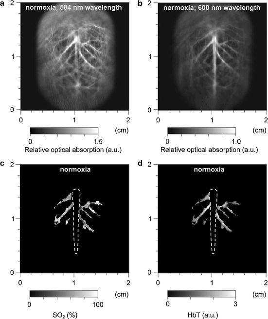
Fig. 2

Noninvasive spectroscopic photoacoustic imaging of HbT and SO₂ in the cerebral cortex of a rat brain. (a) and (b) Brain images generated by 584 and 600 nm laser light, respectively; (c) and (d) image of SO₂ and HbT in the areas of the cortical venous vessels (Reproduced from Wang et al. [59])

3 Principles of PAT Image Reconstruction

In the remainder of this chapter, we describe some basic principles that underlie image reconstruction in PAT. We begin by considering the image reconstruction problem in its continuous form. Subsequently, issues related to discrete imaging models that are employed in iterative image reconstruction methods are reviewed.

A schematic of a general PAT imaging geometry is shown in Fig. 3. A short laser or RF pulse is employed to irradiate an object and, as described earlier, the thermoacoustic effect results in the generation of a pressure wavefield p(r, t). The pressure wavefield propagates out of the object and is measured by use of wideband ultrasonic transducers located on a measurement aperture $\Omega _{0} \subset \mathbb{R}^{3}$ , which is a 2D surface that partially or completely surrounds the object. The coordinate $\mathbf{r}_{0} \in \Omega _{0}$ will denote a particular transducer location. Although we will assume that the ultrasound transducers are point-like, it should be noted that alternative implementations of PAT are being actively developed that employ integrating ultrasound detectors [24, 49].

Fig. 3

A schematic of the PAT imaging geometry

PAT Imaging Models in Their Continuous Forms

When the object possesses homogeneous acoustic properties that match a uniform and lossless background medium, and the duration of the irradiating optical pulse is negligible (acoustic stress confinement is obtained), the pressure wavefield p(r ₀, t) recorded at transducer location r ₀ can be expressed [65] as a solution to Eq. (9):

$\displaystyle{ p(\mathbf{r}_{0},t) = \frac{\beta } {4\pi C_{p}}\int _{V }d^{3}\mathbf{r}\,A(\mathbf{r}) \frac{d} {dt} \frac{\delta \left (t -\frac{\vert \mathbf{r}_{0}-\mathbf{r}\vert } {c_{0}} \right )} {\vert \mathbf{r}_{0} -\mathbf{r}\vert }, }$

(21)

where c ₀ is the (constant) speed of sound in the object and background medium. The function A(r) is compactly supported, bounded, and nonnegative, and the integration in Eq. (21) is performed over the object’s support volume V. Equation (21) represents a canonical imaging model for PAT. The inverse problem in PAT is to determine an estimate of A(r) from knowledge of the measured p(r ₀, t). Note that, as described later, the measured p(r ₀, t) will generally need to be corrected for degradation caused by the temporal and spatial response of the ultrasound transducer.

The imaging model in Eq. (21) can be expressed in an alternate but mathematically equivalent form as

$\displaystyle{ g(\mathbf{r}_{0},t) =\int _{V }d^{3}\mathbf{r}\;A(\mathbf{r})\;\delta \left (t -\frac{\vert \mathbf{r}_{0} -\mathbf{r}\vert } {c_{0}} \right ), }$

(22)

where the integrated data function g(r ₀, t) is defined as

$\displaystyle{ g(\mathbf{r}_{0},t) \equiv \frac{4\pi C_{p}c_{0}} {\beta } t\,\int _{0}^{t}dt^{{\prime}}\;p(\mathbf{r}_{ 0},t^{{\prime}}). }$

(23)

Note that g(r ₀, t) represents a scaled version of the acoustic velocity potential ϕ(r ₀, t). Equation (22) represents a spherical Radon transform [22, 43] and indicates that the integrated data function describes integrals over concentric spherical surfaces of radii c ₀ t that are centered at the receiving transducer location r ₀. When these spherical surfaces can be approximated as planes, which would occur when imaging sufficiently small objects that are placed at the center of the scanning system, Eq. (22) can be approximated as a 3D Radon transform [30, 31].

Universal Backprojection Algorithm

A number of analytic image reconstruction algorithms [22, 34, 64, 65] for PAT have been developed in recent years for inversion of Eq. (21) or (22). A detailed description of analytic algorithms will be provided in Mathematics of Photoacoustic and Thermoacoustic Tomography. However, the so-called universal backprojection algorithm [64] is reviewed below.

The three canonical measurement geometries in PAT employ measurement apertures $\Omega _{0}$ that are planar [66], cylindrical [67], or spherical [61]. The universal backprojection algorithm proposed by Xu and Wang [64] has been explicitly derived for these geometries. In order to present the algorithm in a general form, let S denote a surface, where $S = \Omega _{0}$ for the spherical and cylindrical geometries. For the planar geometry, let $S = \Omega _{0} + \Omega _{0}^{{\prime}}$ , where $\Omega _{0}^{{\prime}}$ is a planar surface that is parallel to $\Omega _{0}$ and the object resides between $\Omega _{0}$ and $\Omega _{0}^{{\prime}}$ .

It has been verified that the initial pressure distribution $p(\mathbf{r},t = 0) = \Gamma A(\mathbf{r})$ can be mathematically determined from knowledge of the measured p(r ₀, t), $\mathbf{r}_{0} \in \Omega _{0}$ , by use of the formula

$\displaystyle{ p(\mathbf{r},t = 0) = \frac{1} {\pi } \int _{S}dS\int _{-\infty }^{\infty }dk\;\tilde{p}(\mathbf{r}_{ 0},k)\,\left [\mathbf{n}_{0}^{S} \cdot \nabla _{ 0}\tilde{G}_{k}^{(in)}(\mathbf{r},\mathbf{r}_{ 0})\right ], }$

(24)

where $\tilde{p}(\mathbf{r}_{0},k)$ denotes the temporal Fourier transform of p(r ₀, t) that is defined with respect to the reduced variable $\bar{t} = c_{0}\,t$ as

$\displaystyle{ \tilde{p}(\mathbf{r}_{0},k) =\int _{ -\infty }^{\infty }d\bar{t}\;p(\mathbf{r}_{ 0},\bar{t})\,\text{exp}(ik\bar{t}). }$

(25)

Here, $\mathbf{n}_{0}^{S}$ denotes the unit vector normal to the surface S pointing toward the source, ∇₀ denotes the gradient operator acting on the variable r ₀, and $\tilde{G}_{k}^{(in)}(\mathbf{r},\mathbf{r}_{0}) = \frac{\text{exp}(-ik\vert \mathbf{r}-\mathbf{r}_{0}} {4\pi \vert \mathbf{r}-\mathbf{r}_{0}\vert }$ is a Green’s function of the Helmholtz equation.

Equation (24) can be expressed in the form of a filtered backprojection algorithm as

$\displaystyle{ p(\mathbf{r},t = 0) =\int _{\Sigma _{0}}d\Sigma _{0}\frac{b(\mathbf{r}_{0},\bar{t} = \vert \mathbf{r} -\mathbf{r}_{0}} {\Sigma _{0}}, }$

(26)

where $\Sigma _{0}$ is the solid angle of the whole measurement surface $\Omega _{0}$ with respect to the reconstruction point inside $\Omega _{0}$ . Note that $\Sigma _{0} = 4\pi$ for the spherical and cylindrical geometries, while $\Sigma _{0} = 2\pi$ for the planar geometry. The solid angle differential $d\Sigma _{0}$ is given by

$\displaystyle{ d\Sigma _{0} = \frac{d\Omega _{0}} {\vert \mathbf{r} -\mathbf{r}_{0}\vert ^{2}} \frac{\mathbf{n}_{0}^{S} \cdot (\mathbf{r} -\mathbf{r}_{0})} {\vert \mathbf{r} -\mathbf{r}_{0}\vert }, }$

(27)

where $d\Omega _{0}$ is the differential surface area element on $\Omega _{0}$ . The filtered data function $b(\mathbf{r}_{0},\bar{t})$ is related to the measured pressure data as

$\displaystyle{ b(\mathbf{r}_{0},\bar{t}) = 2p(\mathbf{r}_{0},\bar{t}) - 2\bar{t}\frac{\partial p(\mathbf{r}_{0},\bar{t})} {\partial \bar{t}}. }$

(28)

Equation (26) has a simple interpretation. It states that p(r, t = 0), or equivalently A(r), can be determined by backprojecting the filtered data function onto a collection of concentric spherical surfaces that are centered at each transducer location r ₀.

The Fourier-Shell Identity

Certain insights regarding the spatial resolution of images reconstructed in PAT can be gained by formulating a Fourier domain mapping between the measured pressure data and the Fourier components of A(r) [6]. Below we review a mathematical relationship between the pressure wavefield data function and its normal derivative measured on an arbitrary aperture that encloses the object and the 3D Fourier transform of the optical absorption distribution evaluated on concentric (Ewald) spheres [6]. We have referred to this relationship as a “Fourier-shell identity,” which is analogous to the well-known Fourier slice theorem of X-ray tomography.

Consider a measurement aperture $\Omega _{0}$ that is smooth and closed, but is otherwise arbitrary, and let $\hat{s} \in \mathbf{S}^{2}$ denote a unit vector on the 3D unit sphere S ². The 3D spatial Fourier transform of A(r), denoted as $\bar{A}(\nu )$ , is defined as

$\displaystyle{ \bar{A}(\nu ) =\int _{V } d\mathbf{r}\,A(\mathbf{r})\,{\mathrm{e}}^{-i\nu \cdot \mathbf{r}}, }$

(29)

where the 3D spatial frequency vector ν = (ν _x, ν _y, ν _z) is the Fourier conjugate of $\mathbf{r}$ . It has been demonstrated [6] that

$\displaystyle{ \bar{A}(\nu = k\hat{s}) = \frac{iC_{p}} {k\beta \tilde{I}(k)}\int _{\Omega _{0}} dS^{{\prime}}\,\left [\hat{n}^{{\prime}}\cdot \nabla \tilde{p}\left (\mathbf{r}_{ 0}^{\,{\prime}},k\right ) + ik\hat{n}^{{\prime}}\cdot \hat{ s}\;\tilde{p}\left (\mathbf{r}_{ 0}^{\,{\prime}},k\right )\right ]{\mathrm{e}}^{-ik\hat{s}\cdot \mathbf{r}_{0}^{\,{\prime}} }, }$

(30)

where $\tilde{p}(\mathbf{r}_{0},k)$ is defined in Eq. (25), dS ^′is the differential surface element on $\Omega _{0}$ , and $\hat{n}^{{\prime}}$ is the unit outward normal vector to $\Omega _{0}$ at the point $\mathbf{r}_{0}^{\,{\prime}}\in \Omega _{0}$ . Equation (30) has been referred to as the Fourier-shell identity of PAT. Because $\hat{s}$ can be chosen to specify any direction, $\bar{A}(\nu = k\hat{s})$ specifies the Fourier components of A(r) that reside on a spherical surface of radius | k | , whose center is at the origin. Therefore, Eq. (30) specifies concentric “shells” of Fourier components of A(r) from knowledge of $\tilde{p}(\mathbf{r}_{0},k)$ and its derivative along the $\hat{n}^{{\prime}}$ direction at each point on the measurement aperture. As reviewed below, this will permit a direct and simple analysis of certain spatial resolution characteristics of PAT.

For a 3D time-harmonic inverse source problem, it is well known [10, 13, 14] that measurements of the radiated wavefield and its normal derivative on a surface that encloses the source specify the Fourier components of the source function that reside on an Ewald sphere of radius $k = \frac{\omega } {c}$ , where ω is the temporal frequency. In PAT, the temporal dependence I(t) of the heating function H(r, t) is not harmonic and, in general, $\tilde{I}(k)\neq 0$ . In the ideal case where I(t) = δ(t), $\tilde{I}(k) = c$ . Consequently, when Eq. (30) is applied to each temporal frequency component k of $\tilde{p}(\mathbf{r}_{0},k)$ , the entire 3D Fourier domain, with exception of the origin, is determined by the resulting collection of concentric spherical shells. This is possible because of the separable form of the heating function in Eq. (6).

Special Case: Planar Measurement Geometry

The Fourier-shell identity can be used to obtain reconstruction formulas for canonical measurement geometries. For example, consider the case of an infinite planar aperture $\Omega _{0}$ . Specifically, we assume a 3D object is centered at the origin of a Cartesian coordinate system, and the measurement aperture $\Omega _{0}$ coincides with the plane y = d > R, where R is the radius of the object. In this situation, $\mathbf{r}_{0}^{\,{\prime}} = (x^{{\prime}},d,z^{{\prime}})$ , $dS^{{\prime}} = dx^{{\prime}}dz^{{\prime}}$ , and $\hat{n}^{{\prime}} =\hat{ y}$ , where $\hat{y}$ denotes the unit vector along the positive y-axis. The components of the unit vector $\hat{s}$ will be denoted as (s _x, s _y, s _z). Equation (30) can be expressed as the following two terms:

$\displaystyle{ \bar{A}(\nu = k\hat{s}) =\bar{ A}_{1}(\nu = k\hat{s}) +\bar{ A}_{2}(\nu = k\hat{s}), }$

(31)

where

$\displaystyle{ \bar{A}_{1}(\nu = k\hat{s}) \equiv \frac{iC_{p}} {kc\beta \tilde{I}(k)}{\mathrm{e}}^{-ikds_{y} }\int \int _{\infty }dx^{{\prime}}dz^{{\prime}}\,\left.\frac{\partial \tilde{p}(x^{{\prime}},y,z^{{\prime}},k)} {\partial y} \right \vert _{y=d}{\mathrm{e}}^{-ik(x^{{\prime}}s_{ x}+z^{{\prime}}s_{ z})}, }$

(32)

and

$\displaystyle{ \bar{A}_{2}(\nu = k\hat{s}) \equiv \frac{-C_{p}\,s_{y}} {c\beta \tilde{I}(k)} \,{\mathrm{e}}^{-ikds_{y} }\int \int _{\infty }dx^{{\prime}}dz^{{\prime}}\;\tilde{p}(x^{{\prime}},d,z^{{\prime}},k)\,{\mathrm{e}}^{-ik(x^{{\prime}}s_{ x}+z^{{\prime}}s_{ z})}, }$

(33)

where, without confusion, we employ the notation $\tilde{p}(x,y,z,k) =\tilde{ p}(\mathbf{r}_{0},k)$ .

It can be readily verified that Eqs. (32) and (33) can be reexpressed as

$\displaystyle{ \bar{A}_{1}(\nu = k\hat{s}) \equiv \frac{iC_{p}} {kc\beta \tilde{I}(k)}{\mathrm{e}}^{-ikds_{y} } \frac{\partial } {\partial y}\bar{\tilde{p}}(ks_{x},y,ks_{z},k)\Big\vert _{y=d} }$

(34)

and

$\displaystyle{ \bar{A}_{2}(\nu = k\hat{s}) \equiv \frac{-C_{p}\,s_{y}} {c\beta \tilde{I}(k)} \,{\mathrm{e}}^{-ikds_{y} }\,\bar{\tilde{p}}(ks_{x},d,ks_{z},k), }$

(35)

where $\bar{\tilde{p}}(\nu _{x},y,\nu _{z},k)$ is the 2D spatial Fourier transform of $\tilde{p}(x,y,z,k)$ with respect to x and z (the detector plane coordinates):

$\displaystyle{ \bar{\tilde{p}}(\nu _{x},y,\nu _{z},k) \equiv \frac{1} {4\pi ^{2}}\int \int _{\infty } dxdz\;\tilde{p}(x,y,z,k)\,{\mathrm{e}}^{-i(x\nu _{x}+z\nu _{z})}. }$

(36)

The free-space propagator for time-harmonic homogeneous wavefields (see, e.g., Ref. [36], Chapter 4.2) can be utilized to compute the derivative in Eq. (34) as

$\displaystyle{ \frac{\partial \bar{\tilde{p}}(ks_{x},y,ks_{z},k)} {\partial y} = ik\sqrt{1 - s_{x }^{2 } - s_{z }^{2}}\;\bar{\tilde{p}}(ks_{x},y,ks_{z},k) = iks_{y}\,\bar{\tilde{p}}(ks_{x},y,ks_{z},k), }$

(37)

where s _y ≥ 0. Equations (34)–(37) and (31) establish that

$\displaystyle{ \bar{A}(\nu = k\hat{s}) = 2\,\bar{A}_{2}(\nu = k\hat{s})\quad \text{for}\quad s_{y} \geq 0. }$

(38)

Equation (38) permits estimation of $\bar{A}(\nu = k\hat{s})$ on concentric half shells in the domain ν _y ≥ 0 and is mathematically equivalent to previously studied Fourier-based reconstruction formulas [29, 66]. Note that A(r) is real valued, and therefore the Fourier components in the domain ν _y < 0 can be determined by use of the Hermitian conjugate symmetry property of the Fourier transform.