Arterial Spin-Labeled MR Perfusion Imaging Techniques

Francesca B. Pizzini, MD, PhD

Marion Smits, MD, PhD

Roman Wesolowski, PhD Eng

Michael Chapell, PhD

Rolf Jager, MD

Henri J. M. M. Mutsaerts, MD

Juan Antonio Hernandez Tamames, MSc, PhD

▪ Introduction

Arterial spin labeling (ASL) is a relatively new technique for MR perfusion assessment that is particularly useful in brain tissues. From a technical point of view, ASL-MRI is essentially a classic tracer experiment where the injected blood-borne tracer has been replaced by a procedure whereby water protons in the blood have been “labeled” on their way to the organ of interest. This labeling is achieved remotely by the application of radio-frequency (RF) waves that effect an inversion of the magnetization of the blood-water in the region where the RF is applied. This is achieved either for all blood within a region (pulsed ASL) or for blood flowing through a plane (continuous ASL), and for brain perfusion, it is usually performed in the neck. Conventional MR imaging can be used to capture this inverted blood signal once it has arrived in the organ, allowing time for it to arrive. However, the image will also contain contribution from the normal soft tissue in the image, which is much larger in magnitude than is the perfusion signal. Hence, the basic ASL experiment contains two images, one with labeling of blood-water and a second without: the subtraction of the two revealing the perfusion. The reliance on an endogenous tracer means that the ASL technique is noninvasive and, for most variants, readily available on existing hardware. However, the small signal magnitude relative to noise in the images and the relatively short “half-life” of the labeled water mean that careful and optimal acquisition and quantification are required.

The primary goal of this chapter is to provide a complete overview of ASL from the technical issues, such as acquisition and quantification, to the clinical application in the brain including neuro-oncology, neurodegeneration, psychiatry, vascular and inflammatory disease, and epilepsy. The final section is focused on common pitfalls in ASL that should be avoided in diagnosis and a procedure to assess quality. A white paper¹ regarding technical aspects of ASL has recently been published, from which technical recommendations in this chapter are drawn.

▪ Arterial Spin Labeling Acquisition

Tissue functions strongly depend on the underlying perfusion, which is the process of supplying tissue cells with nutrients via oxygenated blood from arteries through exchange across the capillary bed; in brain, it is blood-brain barrier (BBB). The measurement of perfusion using MRI has been an active area of research for over 20 years.²

In general, perfusion techniques can be divided into two categories: exogenous and endogenous methods. Exogenous techniques use intravenous contrast agents such as Gd-DTPA (gadolinium diethylenetriaminepentaacetic acid). Endogenous methods use the water protons in arterial blood as the tracer (natural contrast agent). The endogenous MR method is called ASL or, rarely, arterial spin tagging. In ASL, the magnetization of water molecules of the inflowing arterial blood can be labeled by either saturation² or inversion pulses,³,⁴ altering the magnetization of the arterial blood.² Labeled blood then progressively travels through the arteries and arterioles into the capillary bed where the magnetization is exchanged with that in the tissue, as water is a fast and freely diffusible tracer. ASL can be assessed either qualitatively or quantitatively. If two images are acquired, one with labeled blood and a second nonlabeled, then the difference image yields a qualitative map of perfusion. Qualitative measurements result in perfusion-weighted images that are simply a percentage difference between labeled and nonlabeled images. Quantitative measurements typically involve measuring the voxel signal intensity curve at a range of postlabeling delays and fitting to a complete perfusion model.⁵,⁶

ASL sequence consists of two independent parts: labeling and image acquisition. ASL labeling techniques can be classified into continuous (CASL),⁷ pulsed (PASL),⁸ and, recently introduced, a hybrid of both, pseudocontinuous ASL (PCASL).⁹

In continuous ASL, labeling within the tissue of interests reaches a steady state, due to long labeling time. The major advantage of this method is much higher signal-to-noise ratio (SNR) over the pulsed ASL and also simpler quantitative perfusion models. In the PASL technique, a bolus of arterial blood is labeled and passes through the tissue carrying a transient change in signal. Shorter labeling time with a greater efficiency and smaller RF power deposition are the most important advantages of this method,¹⁰ due to which, CASL often requires additional hardware to be employed.

Labeling—Continuous ASL

CASL is the original method for ASL. Proposed in 1992,²,³,¹¹ this method originated from angiography.¹¹,¹² Early techniques employed multiple saturation pulses,² which were then replaced by
the magnetization inversion approach.³ CASL relies on continuous, flow-induced, adiabatic inversion with simultaneous application of magnetic field gradient in the flow direction¹¹ (Fig. 9.1). This adiabatic inversion pulse alone does not carry any amplitude or frequency modulation; therefore, stationary spins are not under the influence of the adiabatic inversion.¹⁰ By implementing concurrently a magnetic field gradient G along the direction of motion, spins located at position r₀ = ωrf will be inverted. The inversion γG is usually applied for 2 to 4 seconds (labeling duration) to ensure the complete filing of vessels and exchange with inverted arterial spins to the imaging slices. The most common spatial placement of the inversion plane is in the vicinity of the circle of Willis or common carotid. Spins are inverted with efficiency α, which must be considered in the quantification process; typical efficiency values range from 80% to 98%.³,¹¹,¹³,¹⁴,¹⁵,¹⁶ and ¹⁷ The acquisition part of the sequence begins after labeling duration and additional postlabeling delay (PLD).

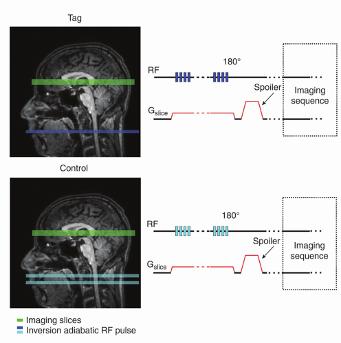Figure 9-1. Schematic diagram of continuous ASL technique. Tag (top) and control (bottom) images are shown with the spatial inversion of tag and control (blue and turquoise, respectively) and imaging slices (green). Pulse sequence for tag and control shown on right.

To estimate perfusion to produce a nonlabel image, the control plane has to be inverted twice, which results in double RF deposition—higher specific absorption rate (SAR), especially problematic in high magnetic fields of 3 T and above. In addition, CASL, with its prolonged train of RF pulses, is particularly sensitive to magnetization transfer (MT) effects resulting in saturation of the static tissue signal in imaging slices. To lower exposure to the excess of SAR, a second RF coil is needed to expand limited coverage, which is an additional, hardware-based disadvantage and difficulty in using this method.

Labeling—Pulsed ASL

Pulsed arterial spin labeling (PASL) denotes a family of sequences and spatial techniques that use a bolus to label the inflowing magnetization. This approach is far less demanding on the hardware and lowers the SAR. The bolus travels through the arteries and arterioles to the capillary bed (recovering with the T1 of blood) where the labeled magnetization is exchanged with unlabelled magnetization of the water in tissue. Once in the tissue, the labeled magnetization then experiences T1 relaxation (T1 of tissue) and eventually recovers and washes out as the fresh, unlabelled blood arrives in the imaging slice. The most commonly used PASL techniques are discussed later in this section. These techniques are described in the form they were initially introduced. Today, however, most of these sequences have variously been optimized and modified, for example, with the addition of pre- and postsaturation pulses.

Figure 9.2 represents the basic sequence for any PASL method; first, we label arterial blood, and then we perform a readout sequence of the desired slice, slices, or volume. In-plane pre- and postsaturation pulses are optional but commonly used in most of the sequences because they limit the effect of poor labeling pulse profile (180 degrees inversion). In-plane saturation becomes more of a requirement at higher fields, where the 180-degree pulses
are even more susceptible to imperfections in their profile and efficiency across the volume. Typically, the in-plane presaturation uses a WET scheme¹⁸ and the postsaturation uses a single sinc pulse.

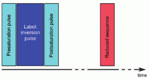Figure 9-2. Schematic diagram of a general pulse sequence of the ASL. Pre- and postsaturation pulses play immediately before and after the label (180 degrees inversion pulse). The red box represents the beginning of the readout sequence.

There is a large number of various pulsed labeling techniques reported in literature, and they all can be used in obtaining ASL images, depending on their availability. This chapter contains only a few most popular approaches.

In the STAR (signal targeting with alternating radiofrequency) technique,⁴ the sequence begins with an in-plane (90-degree) saturation pulse to minimize possible perturbations in the imaging slice from the labeling inversion pulse. The RF pulse is typically followed by an additional spoiler to dephase the magnetization. After the initial saturation, a spatially selective adiabatic inversion pulse is played (Fig. 9.3). The spatial placement of the 180-degree (typically adiabatic hyperbolic secant or frequency offset corrected inversion [FOCI]) inversion¹⁹,²⁰ and ²¹ pulse differs between the tag and control images such that the tag is played below the imaging slice and the control is played above the imaging slice at an equal distance from the center of the slice. This approach avoids discrepancies in static tissue signal between tag and control as a result of the MT effects. However, this original approach would not accurately correct for MT effects away from the isocenter and in particular for multislice acquisitions. A multislice version of EPI STAR has since been developed, which applies two 180-degree pulses back-to-back to act as the control.²² Following the tag/control inversion pulses, at a time equal to the inversion time (TI, equivalent to PLD in CASL and PCASL), a spin echo EPI or gradient echo EPI pulse sequence is typically employed to collect images.

Flow-sensitive alternating inversion recovery (FAIR)²³,²⁴ employs a frequency-selective inversion pulse with and without an accompanying slice-selective gradient (or with a reduced one) to produce tag and control images, respectively (Fig. 9.4). Similar to STAR, the inversion is typically performed using a hyperbolic secant adiabatic pulse (bandwidth of 1 to 5 kHz); for optimal labeling, FOCI pulses are used. The ideal FAIR scheme would employ a 180-degree slab over the imaging volume to produce the tag image and over the entire coverage of the coil to produce the control image. Realistically, in the tagging part of the sequence, the selective inversion must cover more than imaging volume due to imperfect pulse profile (side lobes) and the inversion width in the control image is also spatially selective (approximately 4 times the width of the tagging part) (Fig. 9.4), allowing shorter TR (repetition time). In addition, often, a head-only coil is used for the labeling. Under such circumstances, limiting the inversion pulse width in the control sequence is vital to avoid signal drop-off due to the coil efficiency and to assure arrival of the fresh, noninverted blood at the beginning of the following tagging sequence. FAIR is resistant to MT effects with respect to the imaging slice if slices are centered at zero offset frequency. Again, the image acquisition is obtained following the TI typically using one of the fast imaging sequences.

QUIPSS II (also Q2TIPS)²⁵,²⁶ is very similar to the FAIR technique, only the labeling cutoff is achieved by employing a series of spatially selective saturation pulses applied just prior to image acquisition (Fig. 9.5). The pulses are placed underneath the imaging slab providing a clear finishing edge of the inflowing labeled blood bolus.

Labeling—Pseudocontinuous ASL

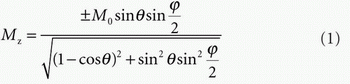
More recently, a hybrid of CASL and PASL techniques, PCASL, has been developed.⁹ Figure 9.6 shows a schematic representation of PCASL tag and control conditions. This method uses rapidly repeated RF pulses in place of the continuous RF and, therefore, overcomes the problems of needing two RF coils or exceeding a safe SAR and is advantageous for scanning as it provides a relatively higher SNR. After repeated application of RF pulses, the magnetization reaches a steady state. The z-component of the magnetization, M_z, in the steady-state conditions is dependent on the flip angle of the RF pulse, θ, and the phase shift experienced during the time between pulses, φ:

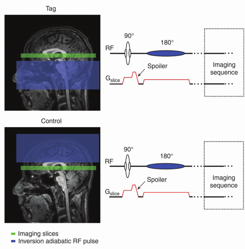Figure 9-3. Schematic diagram of the traditional STAR labeling technique. Tag (top) and control (bottom) images are shown with the spatial inversion of both labeling conditions (blue) and imaging slices (green). Schematics of the radio frequency (RF) and slice-selective gradient of the sequence are shown. It can be seen that gradients are identical for tag and control resulting in equal eddy current effect. Here, the frequency offset is alternated tag and control conditions (blue).

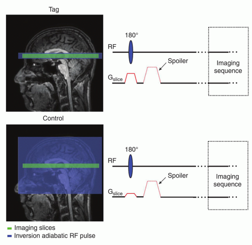Figure 9-4. Schematic diagram of the FAIR labeling technique. Tag (top) and control (bottom) images are shown with the spatial inversion of both labels (blue) and imaging slices (green). Schematics of the RF and slice-selective gradient are shown on the right. The gradient amplitude can be seen to alternate between tag and control conditions.

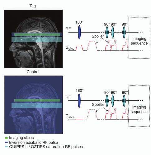Figure 9-5. Schematic diagram of QUIPPS II (Q2TIPS) technique. Tag (top) and control (bottom) images are shown with the spatial inversion of both labels (blue) and imaging slices (green). QUIPPS II (Q2TIPS) saturation slabs are presented in turquoise. Schematics of the RF and slice-selective gradient are shown on the right. The gradient amplitude can be seen to alternate between tag and control conditions.

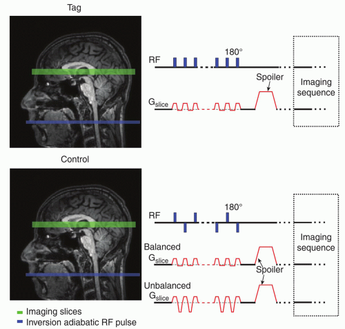Figure 9-6. Schematic diagram of pseudocontinuous ASL technique. Tag (top) and control (bottom) images are shown with the spatial inversion of tag and control (blue) and imaging slices (green). Schematic representation of the RF pulses and the slice gradient of the sequence for tag and control shown on the right. Control condition indicates two variations of the sequence: balanced and unbalanced (marked in the figure).

Similarly to CASL, the image acquisition sequence begins after labeling duration and PLD.

Readout

One of the most popular readout sequences used for ASL is EPI (echo planar imaging).²⁷ This is due to EPI being a method of rapid acquisitions, and it is essential to acquire the image before the label decays. However, alternative acquisition methods may be used, such as 3D-GRASE (gradient and spin echo).²⁸ The advantage of this sequence is that it acquires a 3D volume in a single shot, reducing the slice-dependent variation in perfusion signal due to differences in acquisition delays that occurs with 2D multislice methods. It also provides increased SNR compared to 2D acquisitions. However, it is generally limited to coarse in-plane resolution to reduce off-resonance effects or limited slice thickness to reduce through-slice decay and blurring. Although blurring can be reduced by introducing segmentation in z-plane, there are fewer full-volume images acquired, which makes this sequence very sensitive to motion artifacts. 3D RARE (Rapid Acquisition Relaxation Enhanced)²⁹ with spiral readout trajectory³⁰,³¹ has reduced sensitivity to motion artifacts due to oversampling of the center of the k-space, but can introduce in-plane blurring (resonance offset).³²

Alternatively, more structural-based readout sequences can be used, such as TurboFLASH³³ and TrueFISP,³⁴,³⁵ which have been shown to be advantageous for body ASL applications.

Background Suppression

To improve ASL image quality and reduce physiologic noise contamination, it is very common to use background suppression. Background suppression techniques³⁶ have been proposed to reduce the effects of physiologic noise by suppressing the static signal in ASL data prior to image acquisition. The tag and control images are acquired close to their null point (M_z = 0) in longitudinal (T1) recovery of magnetization by applying a nonselective inversion recovery sequence prior to the ASL acquisition.³⁶ Figure 9.7 shows a schematic representation of a pulse sequence employing background suppression pulses. Background suppression reduces noise from physiologic sources as well as the effects of head motion and other system instabilities of signal intensity. However, the intrinsic suppression of static signal does prevent background-suppressed ASL images being motion corrected.

▪ Analysis and Quantification of ASL

The analysis of ASL data to produce a perfusion image is very simple, requiring only the subtraction of pairs of label and control images. Quantification goes one step further than this and seeks to provide perfusion images on an absolute perfusion scale, so that values in mL/100 g/min can be read from the images. At its most basic, the process of quantification of perfusion would entail three steps:

Subtraction
Kinetic model inversion
Calibration (M_0a calculation)

Subtraction

As noted above, central to the principles of ASL is the subtraction of label and control images, where the “label” images contain signal from static tissue and labeled blood that has been delivered to the tissue:

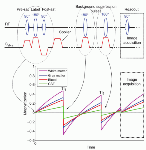Figure 9-7. Top: Schematic of a pulse sequence with two background suppression adiabatic inversion pulses employed. For simplicity, only RF and slice-selective gradient time lines are shown. Bottom: Simulated normalized inversion recovery signals of the longitudinal magnetizations for various brain tissues (white matter, gray matter, blood, and CSF) with two background suppression pulses applied at times TI₁ and TI₂.

This accounts for the labeling process “inverting” the signal from the blood and assumes that (in the ideal case) this “inversion” is 100% efficient. The “control” image, in the absence of the labeling process, consists (ideally) of the same static tissue as well as unlabeled blood:

Subtraction of these two, often referred to as tag-control subtraction, then produces:

This “difference” image is a direct measure of the delivery of blood to the tissue and thus perfusion; a brighter voxel will have had more blood delivered in any given time period (see below).

Compared to the tissue signal, the “blood” signal is small, approximately 1% to 2%. Hence, routinely multiple pairs of label and control images are acquired; these can be combined by taking the average over all the measurements.

Advanced: Motion and Artifacts

Since ASL relies on subtraction to reveal a difference signal far smaller than the static signal that is common to both label and control images, it is susceptible to motion. Any misalignment between the two images, and thus all those in the full data series, will lead to subtraction artifacts; these are often most visible around the brain periphery. Various postprocessing strategies exist for the correction of motion between image frames; from brain images, these typically rely upon rigid realignment of the images, and these equally can be applied to ASL data. However, issues can arise due to the varying contrast between label and control images, which may be interpreted by the motion correction algorithm as a motion effect that it will attempt to correct. It may be desirable to separately motion correct label and control images within the series and only as a final step seek to align them.

ASL perfusion images are also sensitive to the presence of artifacts within individual images in the series. While acquiring multiple pairs and taking the average improves robustness, an individual image with an artifact can lead to errors in the final difference image. A common solution is to manually reject individual images, or most often difference images, that upon visual inspection exhibit an artifact. This approach can also be taken with regard to motion to reject particularly corrupted images due to large subject motion at a particular time during acquisition. More automated approaches either attempt to identify these outlier images by comparison to others in the series, for example, using a correlation measure, or use a more robust method to take the average across the measurements than the mean.

Kinetic Model Inversion

Subtraction results in a relative perfusion image; the next step toward absolute quantification is to account for the relationship between measured signal and rate of delivery of the label itself. This process can be described by a kinetic model, which at its most general is given by a convolution relationship:

This relationship is widely employed in perfusion measurement and states that the measured signal is scaled by perfusion, f, and given by the convolution of two functions:

AIF(t)—The arterial input function, this describes the delivery of the contrast agent—here labeled blood—to the region of interest (voxel) over time.

R(t)—The residue function, this describes what happens to the contrast agent in the time after its arrival.

To convert from measured signal to perfusion, it is thus necessary to “invert” this equation (this inversion assumes that f does not appear in the residue function, which is not true of some more advanced ASL kinetic models—see below).

Various perfusion imaging modalities take differing approaches to the determination of AIF(t) and R(t), including attempting to directly measure them from the data or derive population averages. The nature of ASL imaging means that it is typically appropriate to ascribe simple mathematical forms to both, with parameters that can be determined from the acquisition protocol.

The Arterial Input Function

ASL creates contrast by the RF inversion of blood prior to its entry to the imaging region. This ideally creates a well-defined bolus of labeled blood, and thus, signal at the labeling region takes the form of a boxcar (or “top hat”) function. The duration of the boxcar is determined from the labeling scheme used: for PCASL (CASL), it is simply the labeling duration; for PASL, a spatially defined region of blood will be labeled and normally limited by the spatial extent of the labeling coil; thus, the bolus duration is unknown. For sufficiently short inflow time, it might be appropriate to ignore this parameter. However, more usually where a QUIPPS II or Q2TIPS scheme has been applied, the bolus duration will be defined by the time at which saturation is applied.

By the time the label has reached the measurement region, the label will have decayed due to T1 decay and this needs to be accounted for in the AIF shape. This is where the PASL and PCASL forms of ASL differ: for PASL, some blood is labeled more distally and thus takes longer to arrive in the imaging region; hence, it sees greater T1 decay, and the T1 decay effect is dependent upon the inflow time; for PCASL (and CASL), all blood is labeled at the same distance from the imaging region, and thus, T1 decay effects are only determined by the time of arrival: often called the bolus arrival time (BAT). It is usual in the simplest experiment to assume that this arrival time is negligible.

Finally, the magnitude of the AIF needs to be defined; this is the “concentration” of the label, which is related to the equilibrium magnetization of the arterial blood that was inverted: M_0a. As we have seen above, ASL takes the difference between label and control images so that the magnitude would ideally be twice M_0a. It is also necessary to take the efficiency of the inversion process, α, into account normally using values determined for a typical ASL experiment using the same labeling scheme (see Table 9.1).

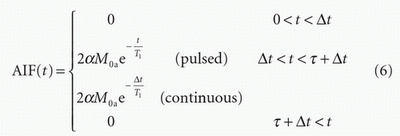
where Δt is the time it takes the blood to travel from the labeling region to the region of interest, BAT, and t is the duration of the labeled bolus. Figure 9.8 illustrates these two input functions. In the simplest case, BAT is ignored, particularly if the inflow time is sufficiently long that its effect on the final measurement is small. The bolus duration is equal to the labeling duration for PCASL; for PASL, it will be determined by the size of the labeling region. However, where QUIPSS II has been used to limit the bolus duration, this parameter will be known.

TABLE 9.1 Recommended Parameters for Quantification, Taken from Ref.¹

Parameter	Value
λ	0.9 mL/g
T1 at 3.0 tesla^a	1,650 ms
T1 at 1.5 tesla^a	1,350 ms
α for PCASL	0.85
α for PASL	0.98
^aThese are based on measured values for arterial blood.

The Residue Function

The residue function describes what happens to the label once it arrives in the measurement region—for a perfusion image, this would be the individual voxels. The simplest assumption is that labeled blood remains with the region; this is predicated on the basis that since the label is created by RF inversion of blood water protons and that water is in rapid exchange between blood and (the much larger volume of) tissue. Thus, as a first approximation, all the labeled blood water that arrives rapidly transfers into the tissue where it remains. However, at the same time, the label continues to decay with time constant T1.

Figure 9.8 illustrates this residue function. Any venous outflow has been ignored here since it is assumed that this will be insignificant compared to the effects of the T1 decay process. This model treats the ASL signal as having entered a single “well-mixed” compartment.³⁷

Kinetic Model

The final model of the signal using the arterial input and residue functions above is shown in Figure 9.8. From this, it can be seen that perfusion simply scales the magnitude of the difference signal; thus, the “inversion” of the model is simple—as long as the effect of the other parameters can be accounted for. The early stages of the time course of the difference signal are very sensitive to BAT, hence the recommendation, for the simplest ASL acquisition, to use a long inflow time so that the signal is measured in the tail end of the curve, which is relatively insensitive to this parameter. Note also that PCASL is less sensitive to BAT than PASL and that the duration of the bolus determines both the amount of signal available and how late the measurement time needs to be to avoid sensitivity to BAT.

Inversion

These simple models can be “inverted” to give the following relationships between signal and perfusion:

PCASL:

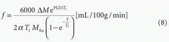
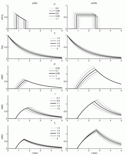Figure 9-8. Examples of functional forms of the ASL signal for both pASL and pcASL acquisitions with variations in some of the key parameters.

PASL (with QUIPSS II):

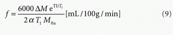
T1 may be chosen based on field strength from Table 9.1 based on measurements in the literature for the T1 of arterial blood. In some populations or in patients, it may be appropriate to use estimates of T1 that have been acquired in the subject using a quantitative T1 sequence. The factor of 6,000 converts the units from
mL/g/s to the conventional mL/100 g/min. For an acquisition that is composed of multiple 2D slices, it will be necessary to use an appropriate PLD or TI for each slice, taking into account the time taken to acquire any previous slices.

Advanced

The simple kinetic model considered above can be extended to incorporate various other processes that affect the quantification of perfusion using ASL:

Arrival Time

Labeled blood will take some time to travel from labeling region to the region of interest, and this delay will also be different across the organ due to the length of different vascular pathways. This can be accommodated into the AIF through the inclusion of an arrival time parameter, as has been illustrated in the definition of the AIF above.³⁷

Venous Outflow

A simple model for venous outflow is to assume that labeled blood leaves the voxel having reached equilibrium with the tissue at a rate determined by perfusion. This can be included within the residue function³⁷,³⁸ but typically has a small effect on the shape of this function.

T1 Decay Rates

Typically, the T1 decay in tissue is shorter than in blood, and thus, separate T1 values might be defined for the AIF and residue functions.³⁷

Further effects that can in theory be modeled, but are harder practically to measure and thus account for, include dispersion of the bolus of labeled blood water during transit through the vasculature³⁹,⁴⁰ and the rate at which labeled blood water exchanges into the tissue.⁴¹,⁴²

These more complex models of ASL kinetics typically require extra information to permit the computation of parameters associated with the effects they describe. For example, the inclusion of arrival time requires a measurement of bolus arrival in the voxel. This information can be obtained by sampling the ASL signal at a range of inflow times and thus sampling the kinetic signal itself. The process of model “inversion” then becomes one of model fitting— minimizing the error between the (noisy) data and the model by the judicious choice of the model parameters, most commonly performed using a sum-of-squares-error measure.

Calibration (M_0a Calculation)

A key parameter of the AIF that is required to quantify perfusion is the equilibrium magnetization of arterial blood that has been labeled: effectively the “concentration” the ASL tracer. Unlike the relative perfusion, this cannot be determined from the difference images. However, it is possible to calculate a surrogate measure of the equilibrium magnetization in the tissue at every voxel, M_0t, and relate this to the equivalent arterial blood magnetization, M_0a. Most commonly, a separate proton density image (with long TR) will be acquired and used to quantify M₀ of tissue— this is generally reasonable if TR > 5 seconds.¹ For shorter TR, for example, using the control image itself, a correction may be applied:

where T_1,tissue is the T1 of tissue—typically gray matter values would be used.

Since the proton density of tissue differs from that of arterial blood, a correction is introduced based on the partition coefficient, λ:

A single whole brain partition coefficient of 0.9¹ may be assumed.

Advanced

The above approach makes a voxelwise calculation of M_0a that can then be applied in the quantification using the equations given above. However, noise from the proton density image will be imported into the perfusion quantification. An alternative approach is to quantify M_0t in a region of homogenous composition, for example, a region of white matter (WM) or CSF. An average taken across the region (to reduction corruption by noise) allows a single global value of M_0a to be calculated, theoretically reflecting the single value of M_0a for the labeled blood bolus. The region used may be defined manually or through automated segmentation of a structural image. The disadvantage of this approach is that it will not correct for variations in coil sensitivity, for example, in segmented acquisitions, and thus, a separate sensitivity image may be required or sensitivity correction applied in the acquisition.

While M_0a is required to quantify perfusion, a measurement of T1 might also be valuable (to account for its variation within the brain). The measurement of the two can be combined using a saturation recovery sequence. A series of measurements at different TIs permits both M_0t and T_1t to be determined from the data. In some cases, saturation recovery has been combined with the main ASL acquisition and inflow times, allowing a single acquisition to be used to collect all the required data, for example, the QUASAR sequence.⁴³

Partial Volume Effects

Issues surrounding the presence within an individual voxel of multiple tissue types are present in a wide range of MR imaging methods. For perfusion imaging with ASL, the effects of partial voluming relate both to the boundary between CSF and tissue and between GM and WM. The former is more obvious because CSF will have no perfusion and thus should contribute no ASL difference signal—leading to underestimation of perfusion in voxels containing a partial volume of CSF. However, a mixture of white and gray matter is also important because the two tissue types have substantially different perfusion characteristics. The main difference is the lower perfusion in WM. It also exhibits a shorter T1 as well as a longer arterial arrival time (AAT).

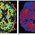
The different perfusion properties substantially dictate the form of the normal ASL perfusion image, meaning that a lot of the features reflect the underlying variations in structure of the brain as shown in Figure 9.9.

It is possible using segmentation methods, applied typically to T1- or T2-weighted images, to estimate the partial volume contributions within voxels of an image. It is then possible to write down the contribution of each “tissue” type to the ASL signal:

These can be used to correct for the effects of partial voluming, and a number of strategies have been proposed:

Rescaling The simplest method is to rescale the values in the subtracted image based on the estimated proportions of gray matter (GM) and WM.⁴⁴ Since the actual contribution (i.e., perfusion) of both GM and WM is unknown and we have only one measurement within the voxel, it is necessary to define one further constraint to solve the equation above for the difference image. This can be achieved by assuming the ratio of GM and WM perfusion.
This in turn is the main drawback of this approach since it does not allow for variations in this ratio throughout the brain, or that a suitable value for this ratio is not well established.

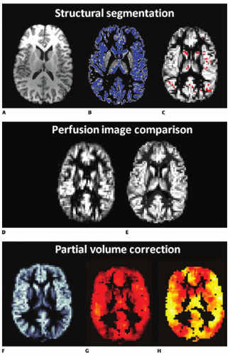Figure 9-9. Examples of partial volume effects in ASL and their correction. A typical structural image (A) has been segmented into tissue types and GM contributions greater than 90% highlighted (B). Once these partial volume estimates have been transformed into the same resolution as ASL data, very few voxels contain a high proportion (>90%) of GM (C). The look of perfusion images is often highly dependent upon the underlying structure: Compare a typical ASL perfusion image (D) with one created using a set of partial volume estimates and spatially constant GM and WM (60 and 20 mL/100 g/min respectively) perfusion values (E). Partial volume correction can be applied using a structural scan: GM partial volume estimates (F) (along with WM) have been used to correct the ASL perfusion image (G) to create a GM perfusion image (H).

Linear regression⁴⁵ takes a different approach for solving the equations above. Instead of assuming a fixed ratio between different tissue types, it assumes that perfusion varies smoothly in the brain, and thus, it is approximately reasonable to assume that GM and WM perfusion in neighboring voxels will be identical. The method proceeds by, for each voxel, choosing a neighborhood of voxels and solving a set of simultaneous equations based on the equations above across all of them to arrive at the GM and WM contributions. The size of the neighborhood needs to be chosen manually with larger sizes leading to more stable solutions. The strength of the approach is that it does not rely upon an assumed ratio, but it does introduce further smoothness into the perfusion images, which gets more substantial as the size of the neighborhood used increases.

Advanced

More advanced methods based on similar principles to the linear regression method have been proposed, including a method that attempts to adaptively determine the appropriate neighborhood for the calculations directly from the data,⁴⁶ as illustrated in Figure 9.9. Additionally, partial volume correction methods have been applied to multidelay ASL exploiting the different kinetics of GM and WM (T1 values and AAT) to increase sensitivity, thus accuracy of the perfusion estimates.⁴⁶ An issue for partial volume correction is the accurate estimation of the partial volume values at the first place. These are normally most accurately achieved using high-resolution structural scans and preferably using a combination of T1- and T2-weighted images. However, these estimates then need to be transformed into the same resolution as that of the ASL data, requiring a good registration between the ASL and structural images. Additionally, typically, the ASL and structural images will have been acquired with different readouts leading to them having different distortions, particularly around the ventricles. Thus, while accurate PV estimates can be achieved from high-resolution images, errors will be introduced in the transformation process. Alternatives such as a segmentation of an image matching the ASL data, such as the raw control or calibration images, have been explored since these avoid transformation and distortion issues.⁴⁷ However, these are far more difficult to segment with any degree of accuracy.

▪ Neuro-Oncologic Disease

MR perfusion imaging is extensively used in the context of neurooncological disease, where vascularisation and vascular proliferation are prominent features for tumour characterisation and grading. Increased vessel diameter and number of vessels in brain tumors lead to local increases in cerebral blood volume (CBV), which is usually assessed with T2-/T2^★-weighted dynamic susceptibility contrast (DSC) MR imaging. DSC MR imaging is used in the clinical routine to differentiate types of brain tumors and metastases,⁴⁸,⁴⁹ and ⁵⁰ to grade neuroepithelial brain tumors,⁵¹,⁵²,⁵³ and ⁵⁴ and to distinguish tumor progression from treatment effects.⁵³,⁵⁵,⁵⁶,⁵⁷ and ⁵⁸

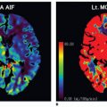
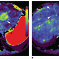
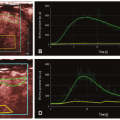
There are now several studies that have evaluated ASL perfusion imaging in brain tumors.⁵⁹,⁶⁰ and ⁶¹ ASL has several advantages over contrast agent perfusion techniques for the assessment of neuro-oncologic disease. Its noninvasiveness is often—but unjustly—dismissed in this context, because contrast agent administration is generally required in the evaluation of brain tumors, in which contrast enhancement is considered a key diagnostic feature. Contrast-enhanced perfusion imaging however requires a larger-bore intravenous cannula for, as well as a larger volume of contrast administration than conventional contrast-enhanced MR imaging. Especially in the pediatric population and in patients on or after chemotherapy, with difficult intravenous access, as well as patients with renal insufficiency, non-contrast-enhanced perfusion imaging can still be considered advantageous. A methodologic advantage is the fact that ASL is insensitive to the disturbing effects of contrast agent leakage occurring with disruption of the BBB. Extravasation of contrast agent to the extravascular compartment reduces the T2-/T2^★-weighted signal due to T1 shortening and as such leads to an underestimation of CBV with T2-/T2^★-weighted contrast-enhanced perfusion MR imaging techniques (Fig. 9.10). Furthermore, ASL is not sensitive to susceptibility artifacts, such as due to hemorrhage (Fig. 9.11), metallic surgical material (Fig. 9.12), or air-tissue interfaces (Fig. 9.13).

In a study comparing a multitude of perfusion techniques (T2-/T2^★-weighted DSC and T1-weighted dynamic contrastenhanced perfusion MR imaging, H₂¹⁵O positron emission tomography (PET), and pulsed ASL), Lüdemann et al.⁶⁰ demonstrated a nearly linear correlation between the various parameters assessed with these techniques. The estimated values for tumor perfusion on the other hand were significantly different between the techniques and can therefore not be compared or interchanged. Relatively small tumor perfusion ratios were obtained with H₂¹⁵O PET and T2-weighted DSC, while T1-weighted DCE perfusion MR imaging seemed to overestimate tumor perfusion. The pulsed ASL and T2^★-weighted DSC yielded median estimation of tumor perfusion. Pulsed ASL, however, had the largest statistical uncertainty and failed to represent very highly perfused tumor regions.

Although it is CBV that is the most widely used parameter in the context of brain tumor perfusion imaging, cerebral blood flow (CBF) measurements with ASL seem to yield similar results.⁶²,⁶³ In contrast-enhancing brain tumors, CBV measured with T2^★-weighted DSC perfusion MR imaging was found to significantly correlate with CBF measured with pseudocontinuous ASL (Pearson correlation coefficient r = 0.70).⁶⁴ Furthermore, tumor CBF measurements with T2^★-weighted DSC perfusion MR imaging correlate with those obtained with ASL,⁵⁹,⁶⁵ while CBV values calculated from ASL data were found to correlate with those obtained with T2^★-weighted DSC perfusion MR imaging⁶⁶ (Fig. 9.14).

Tumor Diagnosis

The differential diagnosis of certain intra-axial brain neoplasms can be challenging, but may have important—presurgical—therapeutic implications. ASL studies of brain tumor diagnosis are still relatively scarce and overall retrospective in nature. An important finding reported by Noguchi et al.⁶⁷ is that ASL measurements correlated with the relative vascular density as well as cellular proliferation in a wide variety of brain neoplasms (Fig. 9.15).

In a retrospective study comparing 19 patients with primary central nervous system lymphoma (PCNSL) to 37 patients with glioblastoma multiforme, Yamashita et al.⁶⁸ demonstrated a significantly lower absolute and relative blood flow in PCNSL. The same research group also looked at the differentiation between hemangioblastoma and metastases in the brain and found that tumor blood flow in hemangioblastoma was more than double that of most metastases.⁶⁹ A renal cell carcinoma metastasis, however, was found to have even higher blood flow than hemangioblastoma. Both these studies support the notion that ASL measurements reflect histopathological tumour characteristics.

Tumor Grading

Primary brain tumors are not only classified but also graded to predict biologic behavior and to guide therapeutic management. The World Health Organization (WHO) grading system is the most widely used and is based on the tumor’s cellularity, mitosis, necrosis, pleomorphism, and vascular proliferation. Vascular proliferation is the basis of the radiologic features of high-grade tumor, namely, enhancement after contrast administration and increased tumor perfusion. Diagnostic accuracy of tumor grading based on contrast enhancement is only moderate, which is significantly improved with perfusion imaging.⁵¹ The relative CBV (rCBV) is the most widely used parameter obtained with DSC MR imaging for brain tumor grading. The rCBV increase shows a reliable correlation with tumor grade and increased tumor vascularity.⁷⁰ CBF measured with DSC MR imaging performs less well,⁷¹ which may be attributed to both physiologic and methodologic issues. Physiologically, it has been suggested that CBF is not consistently and homogeneously increased in areas of vascular proliferation: arteriovenous shunting, occurring particularly at the tumor margins, leads to CBF increase, but CBF may also be decreased due to the tortuosity and reduced lumen of the newly formed blood vessels.⁷² Methodologically, measurement of CBF requires an arterial input function, which can be difficult to determine with DSC perfusion MR imaging. Previous studies assessing CBF with DSC perfusion MR imaging may therefore have suffered from inaccurate CBF estimation.

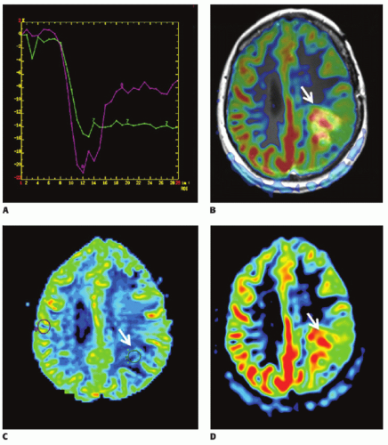Figure 9-10. Enhancing tumor (arrow, B) with leakage of contrast resulting in an underestimation of the rCBV (A, green curve). DSC rCBV maps (arrow, C) fail to identify the high perfusion, visible on the ASL CBF maps (arrow, D). Images courtesy of Dr. Álvarez Linera, Ruber Hospital, Madrid (ES).

In studies assessing ASL for tumor grading, CBF measurements were found to distinguish high- (grades III and IV) from low (grades I and II)-grade tumors⁴⁸,⁵⁹,⁶⁴,⁷³,⁷⁴ and to correlate with CBV measurements assessed with DSC perfusion MR imaging.⁶⁴ Importantly, however, most studies used relative rather than absolute CBF values. Warmuth et al.⁵⁹ specifically reported that absolute tumor blood flow was less important for tumor grading than tumor blood flow relative to the mean brain perfusion. They suggest that as a “rule of thumb,” mean tumor blood flow of low-grade gliomas is less than the mean CBF, while that of high-grade gliomas is greater than the mean CBF. As with DSC perfusion MR imaging, specificities for distinguishing tumor grades individually (e.g., grades III from IV) are not as high.⁴⁸

Only gold members can continue reading. Log In or Register to continue