Basic Principles of Magnetic Resonance Imaging

Magnetic resonance (MR) imaging has become the dominant clinical imaging modality with widespread, primarily noninvasive, applicability throughout the body and across many disease processes. The flexibility of MR imaging enables the development of purpose-built optimized applications. Concurrent developments in digital image processing, microprocessor power, storage, and computer-aided design have spurred and enabled further growth in capability. Although MR imaging may be viewed as “mature” in some respects, the field is rich with new proposals and applications that hold great promise for future research health care uses. This article delineates the basic principles of MR imaging and illuminates specific applications.

Magnetic resonance (MR) imaging has become the dominant clinical imaging modality with widespread, primarily noninvasive, applicability throughout the body and across many disease processes. This progress of MR imaging has been rapid compared with other imaging technologies and it can be attributed in part to physics and in part to the timing of the development of MR imaging, which corresponded to an important period of advances in computing technology. The history of MR imaging dates from the experiments of Paul Lauterbur in the 1970s and includes the work that resulted in his being awarded the Nobel Prize. Compared to radiography, which develops contrast based upon density, MR imaging probes at least three fundamental parameters and a number of derivative ones. For this reason, exquisite soft tissue differentiation is possible. The flexibility of MR imaging enables the development of purpose-built optimized applications. Concurrent developments in digital image processing, microprocessor power, storage, and computer-aided design have spurred and enabled further growth in capability. Although MR imaging may be viewed as “mature” in some respects, the field is rich with new proposals and applications that hold great promise for future research health care uses.

MR imaging is a modality that richly rewards the clinical practitioner who understands the underlying physics. Compared to other imaging techniques, there are many degrees of freedom in the acquisition parameters for MR imaging. There are opportunities for standardization and also opportunities to tailor protocols to specific disease manifestations and even to specific patients. A variety of artifacts can potentially compromise image quality and their presence can be mitigated or addressed with choices of technique. In MR imaging, there is always an opportunity to trade speed for quality (or vice versa), and the balance point of this compromise may yield an optimum study that maximizes benefit to the patient. The interested reader is encouraged to investigate these topics further in any of several more comprehensive texts.

Spin physics

When the physics of MR imaging is discussed in the classical sense, the fundamental concept is that of “spin” or of “a spin.” Spin refers to a magnetic moment that results from or is associated with a “current loop” created by a spinning charged particle, where the charge resides on the outer surface of the particle. This current can be quantified as

I=q∗v/2πr
I=q ∗ v / 2πr

with q the charge on the particle, r the radius of the particle, and v the tangential velocity of a point on the surface of the particle. For clinical MR imaging, the spin of interest is most often that associated with a proton of water.

The magnetic dipole moment that results is the product of the area of the particle and the current. It is a vector quantity and has direction that is parallel to the angular momentum of the spinning particle. The equation

μ = q / 2m ∗ J

quantifies the dipole moment with J the angular momentum, q the charge and m the mass of the particle.

Spins tend to align with an external magnetic field, in the same way that iron filings align with a magnetic field in free space. There are two preferred alignments for spins, referred to as “up” and “down” relative to the direction of the applied field. A slight energy difference exists between the two orientations, and thus a system of many spins can be characterized by its energy state. Over time, when spins experience an external field, they will align to a lower energy, or equilibrium, state, characterized by the distribution between the up and down states. A stronger field will develop stronger polarization between the two states, and when the external field changes for a given system of spins a process of “relaxation” to the new equilibrium state will transpire. When a large number of spins are considered as a system, the effect described is observed as that of a single magnetic moment with a direction that can vary in three dimensions. The energy transfer processes that underlie this effect are exploited by MR imaging techniques to gain information about the relevant spins.

When spins are “polarized” or aligned by a static external magnetic field, they can be excited as an ensemble by the application of radiofrequency energy and, given a large enough number of spins, the effects can be detected. The size of the ensemble required for detection is also related to the strength of the external field- giving rise to some fundamental tenets of MR imaging: a larger sample gives a better signal, and a larger (stronger) magnet will do the same, all else equal.

The excitation of the spin ensemble is achieved via resonance, which is the familiar phenomenon by which certain systems can be most effectively excited at a certain frequency. A common example of this is experienced when pushing a child on a swing. If every sequential push is performed with a constant force there is a certain frequency of pushing that will result in the largest effective energy transfer and consequently a higher arc for the child/swing system. Pushing faster or slower has a diminished effect. In magnetic resonance, the characteristic frequency depends upon the characteristics of the spin under investigation and the strength of the applied magnetic field as:

f = γ B

where gamma is the gyromagnetic ratio, a fundamental constant for a given spin, and B the field strength. This famous relationship is known as the Larmor equation. Excitation of the spin system through application of energy at the resonance frequency can be shown to be equivalent to exposing the system to an altered magnetic field, eg, one that is perpendicular to the applied external field. The spins respond, as given above, by relaxing toward the (new) equilibrium state that is associated with the altered field. Thus they relax or move toward an axis that is not parallel to the (large) applied static field.

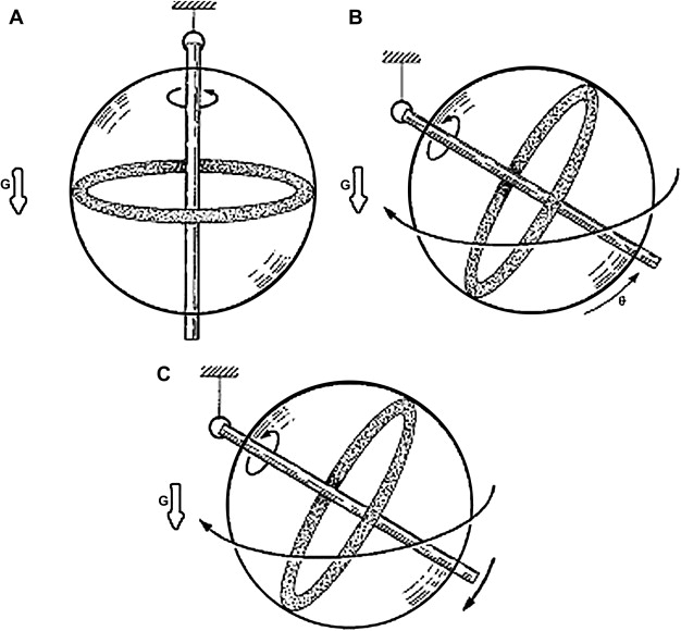
The motion of the vector representation of a spin ensemble toward an equilibrium position is essential to understanding the basis of MR imaging. That motion is precession, analogous to that observed in a gyroscope ( Fig. 1 ). Precession is characterized by the path taken by a spinning object under the influence of an external force, eg, in the case of a gyroscope: gravity. A spinning gyroscope does not behave as it would were it stationary. Instead of falling over in response to gravity, it “spins down” toward a final rest position at a rate related to its mass and spin velocity. Similarly, when a spin system, aligned with the main magnetic field, is exposed through resonance radiofrequency irradiation to an effectively altered field, it will pass from rotation about the axis of the external field to precession around the axis of the effective field. Upon removal of the resonance excitation, the spin system will again experience only the external field and will precess toward its former equilibrium position.

The motions of spins, or, more correctly, ensembles of spins, were elucidated by Bloch and Purcell who for this work shared the Nobel Prize in 1952. Bloch described this motion with a series of coupled differential equations (Bloch equations) that when solved give rise to two exponential relaxation constants known as T1 and T2. The T1 constant is associated with spin–lattice relaxation and describes the exchange of energy between the spin system and the environment. T1 also (or equivalently) describes the longitudinal relaxation along the z-axis. The state of z-magnetization can be normalized to between 1 (equilibrium) and −1. The T2 constant describes the coherence of the spin system, a measure of how “together” the spins are as they rotate. This can be normalized to 1 for the situation where all of the spins are aligned, and to zero when describing a completely random orientation between spins within the system.

A special case of motion of the effective spin vector is seen when the vector rotates perpendicular to the main magnetic field. If the main field is assumed to be oriented in the z-direction as is conventional, this spin rotation is said to be in the x–y plane. With the spins rotating in this manner, it is possible to introduce a coil of wire such that the spins effectively serve as magnets whose lines of flux cut the coil, giving rise to Faraday induction and an induced voltage in the coil. This principle is exploited to obtain the signal associated with the spin behavior at a given time, resulting in data from which an image can be reconstructed.

MR imaging hardware

Principal components that comprise an MR imaging system include: a main magnet, gradient magnets, radiofrequency coils to transmit and/or receive the MR imaging signal, and associated signal processing equipment.

State of the art clinical MR imaging systems typically incorporate a superconducting magnet to produce a relatively large static magnetic field. The function of this magnet is to produce a stable, spatially homogeneous magnetic field over a prescribed volume. Such a magnet may operate at 1.5 Tesla (T), or 15,000 Gauss, which can be compared with the earth’s magnetic field at approximately 0.5 Gauss. Modern magnet systems can also be obtained at 3T and higher fields, and there are also lower-field magnets available, typically at lower cost or for special purposes. Superconducting magnets are cooled by cryogens such as liquid nitrogen and liquid helium and, after the static field is established, they require no electric power to maintain it. Cost, weight, and siting are often important considerations when installing a magnet system. Increased field strength is desirable from the standpoint of signal to noise ratio (SNR) (ie, signal quality) but carries the disadvantages of increased cost largely because of the need for more wire to carry the high current as well as the increased size of the cryostat. In addition, fringe fields must be designed for and the footprint of the device may be large relative to other imaging equipment.

The main magnet will typically incorporate the capability of making small adjustments to the field to achieve the homogeneity necessary for MR imaging. This may be accomplished with secondary magnetic fields known as “shims,” which add to the main field in a spatially inhomogeneous way to correct errors and compensate for engineering factors.

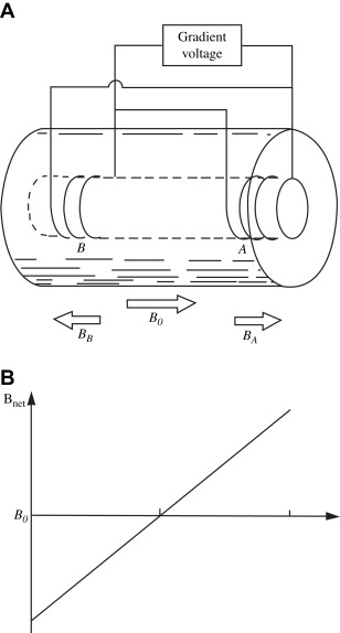
Another kind of secondary magnetic field incorporated for MR imaging is known as a gradient. Gradient coils are electromagnets installed so that when energized, they predictably perturb the main magnetic field along an axis. Thus, in the z-direction, the effective (net) field in the presence of a gradient can be given as

B net = B 0 + Δ B 0 = B 0 + G Z Z

where B ₀is the strength of the main magnetic field, ΔB ₀is the contribution to the effective field from the gradient, G _zis the strength of the gradient in the z-direction, and Z is the distance along the z-axis ( Fig. 2 ). The value G is usually given in mT/m. Referring to the Larmor equation given above, it is seen that in the presence of a gradient, the resonance frequency associated with the sensitive volume of the main magnet varies along the gradient axis. Assuming that the variation of the field along that axis is linear, the frequency variation will also be linear. This observation will form the basis for the MR imaging techniques discussed below.

To obtain three-dimensional images, it is required that at least three gradients be present. An additional practical requirement is that they must be able to be switched on and off very rapidly. The isocenter of the three gradients should be co-located with the isocenter of the main magnet.

Radiofrequency coils are used to excite a particular volume of interest by adding energy to the tissue or material within that volume. They also serve to detect the eventual MR imaging signal. In some applications, both transmit and receive functions are performed by the same coil; in other systems, it is advantageous to employ separate transmit and receive coils. Analogous to the swing example given above, the radiofrequency coils are tuned to the resonance frequency of the spins and thus they are able to add energy in an effective manner to the spin systems. Radiofrequency coils can be constructed with a variety of geometries and they are increasingly built for specific applications. They vary from the large “body coil” that is supplied with many magnet systems and still used for imaging of larger portions of the body, to coils designed for a single finger or perhaps an internal organ. There is a substantial advantage to tailoring the size of the coil to the tissue being examined because the signal in the image must only come from the tissue of interest, whereas the noise associated with that image will originate in the entirety of the coil. Because the image quality is related to the SNR, it is apparent that the highest quality will in general be achieved with coil size optimized to the tissue of interest. It is not only possible but also ubiquitous to “trade” speed for quality in MR imaging. Whenever sufficient quality exists in the acquisition, one can opt to image faster while sacrificing a predictable amount of quality, measured as the SNR.

Radiofrequency coils are increasingly provided as arrays of individual coils that are used sequentially during the imaging sequence. This design can be used to increase quality by redundant or semiredundant acquisition of data, or to increase coverage of an area by establishing a coil array with a predominant linear dimension, for example, to image the spine. This is a way of increasing SNR, which can be used to produce images with higher quality or, alternatively, to increase the speed of acquisition.

When voltage is induced in the radiofrequency coil, the voltage is amplified by a receiver and sent through a signal processing train to be stored in a computer. The computer will carry out the reconstruction of an image when sufficient data is obtained. When phased arrays of coils are used, each must be connected to a separate channel for signal processing.

Only gold members can continue reading. Log In or Register to continue