Computerized image analysis is becoming more routine in multiple sclerosis research. This article reviews the common types of task that are performed when producing quantitative measures of disease status, progression, or response to treatment. These tasks encompass uniformity (bias) correction, registration, segmentation, image algebra and fitting, diffusion tensor imaging and tractography, perfusion assessment, and three-dimensional visualization. The aim of these steps is to output reproducible, quantitative assessments of MR imaging scans that can be performed on data generated by the many different scanning sites that may be involved in multicenter studies.
Standard T 1-and T 2-weighting have formed the basis of contrast in most MR images since the clinical utility of these types of scan was demonstrated by showing abnormal morphology or pathology. For diagnostic purposes, a simple dual-echo image allows the radiologist or clinician to assess the number, position, and shape of tissue abnormalities in the brain and spinal cord, all of which are factors in making a differential diagnosis of multiple sclerosis (MS). Lesions that enhance with injectable contrast agents, such as gadolinium diethylenetriamine penta-acetic acid (Gd-DTPA), are most easily seen on T 1-weighted images.
The need to make quantitative measurements of factors that are more subtle, or open to subjective interpretation, has long been recognized, however; for this, computerized analysis makes these sorts of measurement feasible or can assist in reducing any operator bias in the measurement, or even remove it completely. This review summarizes the tasks that are commonly applied in the analysis of MR images so that quantitative results can be presented.
Uniformity (bias) correction
MR images have an arbitrary intensity scale, in which the actual intensity values depend on such factors as the receiver gain setting, sequence parameters (repetition time [TR], echo time [TE]), and tissue type. Furthermore, the intensity of a certain tissue type varies according to its position in the radiofrequency (RF) transmitter and receiver coils, because the RF field and reception properties vary spatially. This intensity nonuniformity (or bias) is most obvious in images acquired using surface receiver coils, such as those used for spinal cord imaging, but it is present in all MR scans.
For quantitative image analysis, which relies on relative intensities, this bias is obviously a problem, and several methods for its correction have been put forward. Ideally, the bias field can be measured at the time of scanning by running extra pulse sequences and then corrected in situ. However, retrospective correction has been investigated by several groups (for a review, see the article by Belaroussi and colleagues ). A basic assumption behind all the retrospective correction methods is that the bias field varies only slowly in space, which is a reasonable assumption, given that the bias field comes mainly from nonuniformities in the RF field. Some methods model the bias field as a sum of smooth polynomial or trigonometric functions, whereas others assume that the bias field is (spatially) piecewise uniform. Other methods integrate the classification of tissue types (eg, white matter, gray matter, cerebrospinal fluid [CSF]) with bias field correction by making the assumption that all tissues in the same class should have a similar intensity.
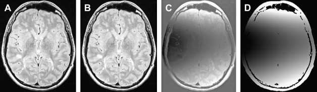
Accurate uniformity correction becomes more important as the number of high-field scanners increases and with the greater use of phased-array receiver coils for head imaging ( Fig. 1 ). Whatever the correction method, uniformity correction is used as a preprocessing step in several applications, particularly in image registration and segmentation.
Registration
Another common task that forms a part of many aspects of image analysis is registration, whereby scans performed at different times are aligned so that the same anatomic locations can be superimposed. The time between scans may be on the order of a second or so, as is seen with functional MR imaging (fMRI), where the registration corrects small amounts of patient movement. The time could be several years, however, in long-term follow-up studies of brain change. The scans may be performed with essentially the same type of contrast (eg, serial T 1-weighted images used to assess atrophy ), or they may have a different contrast or even be collected using a different imaging modality (eg, to integrate data about glucose metabolism using positron emission tomography [PET] scans with high-resolution structural MR imaging scans ).
The process of registering images generally follows a common framework: by an iterative process, a transform is calculated that distorts one scan (the “floating image”) so that it overlays another image (the “base image”) accurately. The parameters of the transform are adjusted to obtain a good match between the two images, and the goodness of the match is evaluated using a “cost function.” The cost function is evaluated over the whole image (sometimes after background removal), and the choice of cost function is dictated by the types of image that are to be aligned. In cases in which the images have similar brightness and contrast (eg, in fMRI time series), the root-mean-square difference or cross-correlation is most appropriate. When images have similar contrast but different absolute intensity ranges (as can occur in images acquired with the same pulse sequence with a long time interval between acquisitions, or on different scanners), the standard deviation of the intensity ratio can be useful.
When images are acquired with different contrast or with different modalities, another class of cost function should be used. These rely on the assumption that although the intensities at the same anatomic location may not be similar across modalities, the intensities are consistent, such that a certain tissue type has a fairly constant intensity for any one modality. When the two images are closely aligned, a two-dimensional (joint) histogram of intensities formed from the images therefore shows sharp peaks, and any misalignment causes a blurring of the histogram, because tissues of different types overlap. Woods and mutual information are among these types of cost function, and they are a measure of this blurring of the joint histogram.
To compare images from different patients, it is necessary to transform them into a standard anatomic space. One such space is based on the brain atlas from the Montreal Neurological Institute (MNI). This was composed by registering the scans from a large sample of control subjects to an average brain that was previously created by transforming a large number of other scans to the standard space of Talairach and Tournoux. The original atlas of Talairach and Tournoux was created from a single rather unrepresentative subject postmortem, which has resulted in some differences between the MNI atlas and the Talairach and Tournoux atlas. Nevertheless, for the purposes of identifying gross anatomic features, the MNI atlas serves well, and the disparity can largely be corrected by applying an additional transform. Therefore, after registering a set of scans to the MNI atlas, it is possible to compare image features across subjects in anatomic space.
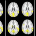
One use of this type of registration to standard space is so-called “voxel-based morphometry” (VBM) analysis, such as that built into the a statistical parametric mapping (SPM) package from the Wellcome Trust Centre for Neuroimaging, London. The goal of VBM is to allow the identification of significant differences in brain tissue across groups of subjects, and it allows the regional and anatomic variation to be visualized, revealing the subtle changes that can occur and the differences among the different MS phenotypes.
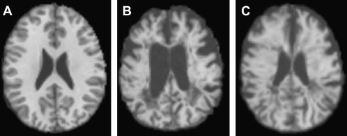
Most registration is done using a simple distortion to transform the image to be registered, such as the affine transform, a property of which is that it always preserves the straightness of straight lines when the transform is applied. This type of linear transform cannot therefore account for the complex differences in the shapes of the brain that occur among individuals; more complex general transforms are needed in this case. Registration using nonlinear transforms is now becoming a much more mature procedure, although it is still compute-intensive. The deformation required to bring about registration is normally modeled as a sum of polynomial, trigonometric, or radially symmetric basis functions. It is used for intersubject registration or for assessing atrophy within a subject. Fig. 2 shows an attempt to register a patient who has MS and a severely atrophied brain to a control subject, first using a simple affine transform and then, with nonlinear registration, using radial basis functions to model the deformation field. Considering the severity of the atrophy, the nonlinear registration produces quite a good anatomic match between the patient and the control.
Registration
Another common task that forms a part of many aspects of image analysis is registration, whereby scans performed at different times are aligned so that the same anatomic locations can be superimposed. The time between scans may be on the order of a second or so, as is seen with functional MR imaging (fMRI), where the registration corrects small amounts of patient movement. The time could be several years, however, in long-term follow-up studies of brain change. The scans may be performed with essentially the same type of contrast (eg, serial T 1-weighted images used to assess atrophy ), or they may have a different contrast or even be collected using a different imaging modality (eg, to integrate data about glucose metabolism using positron emission tomography [PET] scans with high-resolution structural MR imaging scans ).
The process of registering images generally follows a common framework: by an iterative process, a transform is calculated that distorts one scan (the “floating image”) so that it overlays another image (the “base image”) accurately. The parameters of the transform are adjusted to obtain a good match between the two images, and the goodness of the match is evaluated using a “cost function.” The cost function is evaluated over the whole image (sometimes after background removal), and the choice of cost function is dictated by the types of image that are to be aligned. In cases in which the images have similar brightness and contrast (eg, in fMRI time series), the root-mean-square difference or cross-correlation is most appropriate. When images have similar contrast but different absolute intensity ranges (as can occur in images acquired with the same pulse sequence with a long time interval between acquisitions, or on different scanners), the standard deviation of the intensity ratio can be useful.
When images are acquired with different contrast or with different modalities, another class of cost function should be used. These rely on the assumption that although the intensities at the same anatomic location may not be similar across modalities, the intensities are consistent, such that a certain tissue type has a fairly constant intensity for any one modality. When the two images are closely aligned, a two-dimensional (joint) histogram of intensities formed from the images therefore shows sharp peaks, and any misalignment causes a blurring of the histogram, because tissues of different types overlap. Woods and mutual information are among these types of cost function, and they are a measure of this blurring of the joint histogram.
To compare images from different patients, it is necessary to transform them into a standard anatomic space. One such space is based on the brain atlas from the Montreal Neurological Institute (MNI). This was composed by registering the scans from a large sample of control subjects to an average brain that was previously created by transforming a large number of other scans to the standard space of Talairach and Tournoux. The original atlas of Talairach and Tournoux was created from a single rather unrepresentative subject postmortem, which has resulted in some differences between the MNI atlas and the Talairach and Tournoux atlas. Nevertheless, for the purposes of identifying gross anatomic features, the MNI atlas serves well, and the disparity can largely be corrected by applying an additional transform. Therefore, after registering a set of scans to the MNI atlas, it is possible to compare image features across subjects in anatomic space.
One use of this type of registration to standard space is so-called “voxel-based morphometry” (VBM) analysis, such as that built into the a statistical parametric mapping (SPM) package from the Wellcome Trust Centre for Neuroimaging, London. The goal of VBM is to allow the identification of significant differences in brain tissue across groups of subjects, and it allows the regional and anatomic variation to be visualized, revealing the subtle changes that can occur and the differences among the different MS phenotypes.
Most registration is done using a simple distortion to transform the image to be registered, such as the affine transform, a property of which is that it always preserves the straightness of straight lines when the transform is applied. This type of linear transform cannot therefore account for the complex differences in the shapes of the brain that occur among individuals; more complex general transforms are needed in this case. Registration using nonlinear transforms is now becoming a much more mature procedure, although it is still compute-intensive. The deformation required to bring about registration is normally modeled as a sum of polynomial, trigonometric, or radially symmetric basis functions. It is used for intersubject registration or for assessing atrophy within a subject. Fig. 2 shows an attempt to register a patient who has MS and a severely atrophied brain to a control subject, first using a simple affine transform and then, with nonlinear registration, using radial basis functions to model the deformation field. Considering the severity of the atrophy, the nonlinear registration produces quite a good anatomic match between the patient and the control.
Image segmentation
Image segmentation refers to the process of splitting an image into multiple regions (sets of pixels). Segmentation of MRI scans is typically used to identify different types of tissue and their boundaries, such that the volumes or shapes of the individual tissues can be quantified or analyzed further.
Image segmentation can result in a set of regions that, when combined, cover the entire image or a set of object boundaries, such that each of the pixels in a region has some similarity to the others in that object. The similarity may be a simple intensity similarity, may contain information about connectivity within regions, or may be based on some collective shape property. The objective is usually to determine regions that form a set of tissue types, such as white matter, gray matter, or MS lesion.
Measurement of Lesion Volumes
The first and most straightforward use of segmentation in the field of MS research was probably to determine the volume of hyperintense lesions on T 2-weighted images. The segmentation of MS lesions can be done by manually drawing around the boundary of the lesions while showing the scans, slice-by-slice, on a computer display. Using this process, it is quite possible to achieve reasonable reproducibility, but it is labor-intensive. Changes in lesion volumes are used as secondary outcomes measures in clinical trials of new putative treatments for MS, and the lesions may be hyperintense on T 2-weighted images or hypointense on T 1-weighted images (“black holes”). Black hole lesions are thought to represent tissues with more severe cellular damage.
Many workers have addressed the problem of reducing the amount of operator time and improving the reproducibility of the measurement of MS lesion volumes using computer-assisted or fully automated computerized methods. Methods include edge detection and contour following, multiparametric image analysis, template-driven segmentation, and fuzzy connectedness. Of these, the one that is probably most commonly used in clinical trials is one that still relies on operator judgment to identify the individual lesions, but uses an edge detector to find the border of the lesion. The operator visually determines a fairly well-defined portion of the lesion boundary and clicks on it with the computer mouse, an edge detector selects the sharpest part of the boundary, and a contour surrounding the lesion is generated by following a level of isointensity from the initial edge point. This simple method has been shown to improve reproducibility considerably compared to manual outlining.
Many other methods are used by individual research groups for their own clinical and MR imaging research programs. The reproducibilities are often shown to be better than manual identification and outlining, but they are often tested using data from only one MR imaging scanner with specific pulse sequence parameters. It may be that some of these methods do not transfer to the context of multicenter clinical trials because they are sensitive to the subtle differences in images seen between different manufacturers for what are nominally the same pulse sequence parameters.
The most promising approaches are probably based on multiparametric segmentation, whereby information from several scans (eg, the two echoes of a dual-echo sequence and fluid-attenuated inversion recovery [FLAIR]) are combined to segment the lesions based on the position of pixels in an N -dimensional intensity space. The number of dimensions is equal to the number of images and, in principle, the greater the number of images used, the higher is the discriminating power that allows the lesion to be distinguished from other tissues. Fuzzy connectedness can be regarded as an extension of multiparametric methods, but it is a general method for image segmentation in which the object membership of pixels depends on the way they “hang together” spatially in spite of gradual variations in their intensity. For the task of measuring lesion volumes, Udupa and colleagues adopted a three-part procedure. First was the manual identification by the operator of a few typical tissue types on the scan, including MS lesion, normal white matter, normal gray matter, and CSF. Next, the fuzzy connectedness algorithm automatically identified “candidate” MS lesions, and in the final stage, these candidate lesions were presented to the operator, who reviewed them and accepted, rejected, or modified them. Thus, the method implicitly recognized that human operators are good at identifying image features but do not perform well when attempting to delineate the poorly defined borders of the lesions. The operator time required to assess typical image sets from patients who had MS was between 2 and 20 minutes, depending on the number and complexity of the lesions. Another approach based on fuzzy connectedness principles incorporated “domain knowledge” in the form of probability maps, which showed the probability of finding MS lesion tissue at any given anatomic location. This allowed the number of “false-positive” lesions to be greatly reduced, eliminating the need for review. Nevertheless, it was still necessary for the operator to identify each MS lesion manually with a mouse click.
Atrophy
Brain and spinal cord atrophy measures are becoming standard in MS clinical trials, where the loss of neuronal tissue is thought to be an indicator of long-term irreversible tissue damage. This is slightly complicated by the phenomenon of “pseudoatrophy,” whereby the anti-inflammatory effect of some treatments causes a rapid initial loss of brain volume because of a reduction in the amount of excess fluid in the brain. Brain atrophy is a normal feature of aging, with progressive loss of tissue starting in early adulthood. The brain volume is highly variable among individuals, however.
Brain atrophy can be measured cross-sectionally or longitudinally. Cross-sectional measures estimate the total volume of brain tissue. Because the cranial volume and brain size are so variable, however, the results are not easily compared, except in studies of large populations. One way to standardize the measures is to provide a “normalized” brain volume, and there are really two ways to do this. The first is to divide the brain parenchymal volume by the cranial volume, because the cranial volume remains largely fixed throughout adult life. The second is to divide it by the sum of the parenchymal and CSF volumes to form what is known as the brain parenchymal fraction (BPF). As atrophy occurs, the CSF-filled ventricles and sulci enlarge and the BPF reduces; therefore, the BPF is a highly effective measure of the state of atrophy and can be compared across individuals. In longitudinal studies, it is, of course, possible simply to measure the reduction in normalized brain volume over time. More sophisticated approaches first register the scans made at different time points, however; it then becomes possible not only to assess the gross change in tissue volume but to visualize the anatomic location of tissue loss.
Although there are several software packages that can be used to assess atrophy, it is necessary that they have a scan-rescan coefficient of variation (CoV) of around 0.5% or better if they are to be useful for MS research. This allows differences in atrophy rates among groups of subjects to be assessed with relatively small groups (typically 25–50 patients). Virtually all methods use high-resolution T 1-weighted images (multislice spin-echo or three-dimensional [3-D] gradient-echo) as input, wherein the timing parameters are optimized to maximize contrast between the low-intensity CSF and the parenchyma. As a preprocessing step, it is necessary to separate the cranial contents from other tissues, such as scalp, eyes, and facial tissues; this can be achieved in a variety of ways, but one of the most popular is the brain extraction tool, which uses an expanding triangulated surface model that “sticks” to the brain-CSF boundary as it expands from the center of the brain. With sufficient image contrast, segmentation can then be achieved using an intensity threshold to separate brain from CSF. More sophisticated approaches assess gray matter, white matter, and CSF volumes separately, allowing loss of different types of tissue to be assessed; however, this method is prone to errors because of the misclassification of MS lesions as gray matter. Taking this a stage further, a VBM approach allows the identification of the individual brain structures that are particularly subject to atrophy.
It has also been shown that the spinal cord is subject to atrophy, and that the degree of atrophy is related to disability. The cord is, of course, a much smaller structure; because of this, cord atrophy measurements have a much lower reproducibility (larger CoV) than those for the whole brain. A typical approach is to measure the cord area over a fairly limited portion of the cervical region. The cord can be segmented using methods similar to those used in the brain, with a threshold to separate the CSF from the cord parenchyma or using edge detection.
Magnetization transfer
Standard MR imaging detects signal only from hydrogen nuclei (protons) that are “mobile” (contained within a liquid)—if a hydrogen atom is part of a molecule that is large and cannot move about freely, the signal from that hydrogen atom decays too quickly to be seen using a clinical MR imaging scanner. Such protons are found in large molecules (macromolecules), such as those of cell membranes and myelin. The mobile protons are in constant motion, however, and come into regular and intimate contact with the macromolecular protons, and the spin state (the proton magnetization state, which is measured with MR imaging) of the mobile protons can exchange with that of the macromolecular protons. This exchange of magnetization forms the basis of magnetization transfer imaging (MTI).
A magnetization transfer ratio (MTR) image is calculated from a pair of images acquired in an identical way, except that one has extra off-resonance RF pulses applied, which saturates the macromolecular magnetization pool. The MTR is calculated for every corresponding pair of pixels in the two images. If the intensity of the pixel in the image without saturation pulses is M 0 and the corresponding intensity in the image with saturation pulses is Ms , the MTR is as follows:
Related posts:
 The Pathologic Substrate of Magnetic Resonance Alterations in Multiple Sclerosis
 Basic Principles of Magnetic Resonance Imaging
 Brain Atrophy Assessment in Multiple Sclerosis: Importance and Limitations
 MR Relaxation in Multiple Sclerosis
 The Clinical Epidemiology of Multiple Sclerosis
The Use of MR Imaging as an Outcome Measure in Multiple Sclerosis Clinical Trials
The Clinical Epidemiology of Multiple Sclerosis
The Use of MR Imaging as an Outcome Measure in Multiple Sclerosis Clinical Trials
Stay updated, free articles. Join our Telegram channel

Full access? Get Clinical Tree


