, Abas Sabouni2, Travis Desell3 and Ali Ashtari4
(1)
Department of Electrical Engineering, University of North Dakota, Grand Forks, ND, USA
(2)
Department of Electrical Engineering, Wilkes University, Wilkes-Barre, PA, USA
(3)
Department of Computer Science, University of North Dakota, Grand Forks, ND, USA
(4)
Invenia Technical Computing, Winnipeg, MB, Canada
Abstract
This chapter presents a simulation framework and it is used to examine the effectiveness of various asynchronous optimization methods on simulated distributed computing environments. Four benchmark functions were used to evaluate asynchronous versions of differential evolution, genetic algorithms, and particle swarm optimization. Given large-scale homogeneous and heterogeneous computing environments, asynchronous optimization is shown to have superior scalability and performance compared to synchronous implementations, even scaling to potentially millions of processors.
8.1 Simulating Asynchronous Optimization
In order to examine the scalability and performance of the asynchronous optimization methods used for FDTD on hardware far larger than available in a more comprehensive manner, a simulation for these systems was developed. Further, as calculating the objective function for the FDTD application is extremely computationally expensive, it is not feasible to use it for large-scale studies. However, there are a large number of computationally inexpensive test functions that have challenging search spaces with multiple local minima—for example, the Ackley, Griewank, Rastrigin, and Rosenbrock functions as found in related works [1–3].
The Sphere test function was also used as an easy to solve well-formed optimization problems with a single minimum. The optimization test functions used are as follows:
The Sphere function is a simple test function. It has a single minimum with fitness 0 when all input parameters are 0 (see Fig. 8.1). The range of parameters used for this optimization problem was from − 100 to 100.

(8.1)

(8.2)

Fig. 8.1
The Sphere test function with two input parameters (x, y). This is a simple test function with a single minimum at 0,0

Fig. 8.2
The Ackley test function with two input parameters (x, y). This test function has many local minima and a single global minimum at 0,0. Unlike the Griewank and Rosenbrock functions, it converges sharply to the global minimum with a flat external surface

Fig. 8.3
The Griewank test function with two input parameters (x, y). This test function has many local minima and a single global minimum at 0,0. This has a shallow curvature with less pronounced peaks and valleys than the Rosenbrock function
The Ackley function is a more challenging test function with many local minima. There is a single global minimum with fitness 0 when all input parameters are 0 (see Fig. 8.2). It becomes flat near the edges of the problem space and converges sharply to the global minimum. The range of parameters used for this optimization problem was from − 32 to 32.

(8.3)

(8.4)
The Griewank function is another challenging test function with many local minima. It has a shallow curvature and a single global minimum with fitness 0 when all input parameters are 0 (see Fig. 8.3). The range of parameters used for this optimization problem was from − 600 to 600.

(8.5)

(8.6)
The Rastrigin function is similar to the Griewank function. However, it has a less shallow curvature and more pronounced peaks and valleys. The global minimum has a fitness of 0 when all input parameters are 0 (see Fig. 8.4). The range of parameters used for this optimization problem was from − 2π to 2π.
![$$\displaystyle{ f_{\mathrm{rastrigin}}(\mathbf{x}) =\sum _{ i=1}^{N}[\mathbf{x}_{ i}^{2} - 10\cos (2\pi \mathbf{x}_{ i}) + 10] }$$](http://radiologykey.com/wp-content/uploads/2020/04/A305155_1_En_8_Chapter_Equ7.gif)
(8.7)

(8.8)
The Rosenbrock function has no local minima; however, it has a very flat valley with only a single minimum. The minimum has a fitness of 0 when all input parameters are 1 (see Fig. 8.5). The range of parameters used for this optimization problem was from − 30 to 30.
![$$\displaystyle{ f_{\mathrm{rosenbrock}}(\mathbf{x}) =\sum _{ i=1}^{N}[(\mathbf{x}_{ i+1} -\mathbf{ x}_{i}^{2})^{2} + (\mathbf{x}_{ i} - 1)^{2}] }$$](http://radiologykey.com/wp-content/uploads/2020/04/A305155_1_En_8_Chapter_Equ9.gif)
(8.9)

(8.10)

Fig. 8.4
The Rastrigin test function with two input parameters (x, y). This test function has many local minima and a single global minimum at 0,0. It has a steeper curvature with more pronounced peaks and valleys than the Griewank function

Fig. 8.5


The Rosenbrock test function with two input parameters (x, y). This test function has a long flat valley with a single minimum at 1,1
Stay updated, free articles. Join our Telegram channel

Full access? Get Clinical Tree


