, Abas Sabouni2, Travis Desell3 and Ali Ashtari4
(1)
Department of Electrical Engineering, University of North Dakota, Grand Forks, ND, USA
(2)
Department of Electrical Engineering, Wilkes University, Wilkes-Barre, PA, USA
(3)
Department of Computer Science, University of North Dakota, Grand Forks, ND, USA
(4)
Invenia Technical Computing, Winnipeg, MB, Canada
Abstract
This chapter discusses common global optimization methods, such as differential evolution, genetic algorithms, and particle swarm optimization. It provides a survey of the many different strategies utilized in developing and improving these methods. In some sense, global optimization methods are by nature all heuristic-based approaches, as in infinitely sized search spaces with many ill-formed possible local minima it is not possible to analytically provide an optimal solution, as per the no-free-lunch theorem. Because of this, it is not possible to find one single heuristic which will always perform the best for all search spaces. This leads to many various heuristic approaches for different optimization problems. This chapter further provides a survey describing the many hybrid approaches taken to combine different types of both global optimization methods and global optimization methods with local optimization methods in attempts to improve convergence rates and expand exploration. It is important for the reader to recognize that performing global optimization is a balancing act between exploring the search space, to prevent premature convergence to local minima, and exploiting well-performing areas of the search space to quickly converge to a solution. Modifying the heuristics and hybridizing the search methods provide more parameters to tweak to change how the optimization technique explores and exploits areas, which will improve its performance on some problems, but potentially decrease its performance on others.
3.1 Global Optimization Methods
Global optimization methods have been widely researched. In general, they are all variations of Monte Carlo search. These approaches can be divided depending on the type of search space they optimize over. Particle swarm optimization (PSO) and differential evolution (DE) typically operate over a continuous search space, while others like simulated annealing (SA) and tabu search (TS) [1] operate over a discrete (or noncontinuous) search space. Genetic algorithms (GAs) have been well applied to both areas. All these approaches have also been modified or hybridized for use in either search space. Hybridization is also a very popular strategy for enhancing the performance of these global optimization methods, because while they provide effective methods for exploration, finding new potential areas for the global minimum, they often suffer in exploitation, the ability to quickly converge to a minimum within one of these areas. So while hybridizing the various global optimization methods can be an effective method to make one type of global search continuous or discrete (or able to work on a search domain containing both types of parameters), hybridizing these searches with efficient local search methods such as conjugate gradient descent (CGD), the Nelder-Mead simplex method, the proximal bundle method (PBM), or Newton methods provides an effective way to search with both strong exploration and exploitation capabilities.
The remainder of this chapter proceeds by discussing three different global optimization methods used for continuous search spaces. DE, GAs, and PSO are discussed in Sects. 3.2–3.4, respectively. In particular, for each section the global search method is first introduced, and then hybridization strategies are examined.
3.2 Differential Evolution
Differential evolution is an evolutionary algorithm used for continuous search spaces developed by Storn and Price over 1994–1995 [2]. Unlike other evolutionary algorithms, it does not use a binary encoding strategy or a probability density function to adapt its parameters; instead it performs mutations based on the distribution of its population [3]. For a wide range of benchmark functions, it has been shown to outperform or be competitive with other evolutionary algorithms and particle swarm optimization [4].
In differential evolution, an initial population is generated randomly, and each proceeding iteration generates the members of the next population by selecting a parent individual and modifying this parent using a difference vector calculated by a set number of other individuals, and a recombination operator (Fig. 3.1 gives an example of how an individual moves an example two-dimensional search space). The individuals improve monotonically. If the newly generated individual is more fit than the previous individual at its position in the population, the newly generated individual replaces the previous one; otherwise the new individual is discarded. Differential evolution uses the following naming strategy: DE/x/y/z, where DE simply means differential evolution, x indicates how the parent is chosen, y is the number of pairs of individuals chosen to modify that parent, and z is the recombination operator.

Fig. 3.1
A two-dimensional example of how an individual moves in differential evolution
Mezura-Montes et al. study different variants of differential evolution on a broad range of test functions [5]. In general, a new individual x(l + 1) for a new population l + 1 is generated from the individual x(l) from the previous population l. The jth parameter is calculated given p pairs of random individuals from the population l, where  . θ, ϕ, and κ are the user-defined parent scaling factor, recombination scaling factor, and crossover rate, respectively. f(x) is the fitness of individual x. D is the number of parameters in the optimization function. b(l) is the best individual in the population l. They used the following common variants:
 . θ, ϕ, and κ are the user-defined parent scaling factor, recombination scaling factor, and crossover rate, respectively. f(x) is the fitness of individual x. D is the number of parameters in the optimization function. b(l) is the best individual in the population l. They used the following common variants:
best/p/bin selects the best member of the population, adds the sum of the differential between p other pairs of distinct individuals, and performs binomial recombination with an individual to generate its child as follows:
Binomial recombination combines the current individual with the parameters generated by the parent and the pairs by selecting at least one parameter randomly and performing a weighted average using the recombination scaling factor.
![$$\displaystyle\begin{array}{rcl} x(l + 1)_{j} = \left \{\begin{array}{cl} b(l)_{j}^{0} +\phi \sum _{ k=1}^{p}[r(l)_{j}^{1k} - r(l)_{j}^{2k}]&\mbox{ if }r(0,1) <\kappa \mbox{ or }j = r(0,D) \\ x(l)_{j} &\mbox{ otherwise}\end{array} \right.& & {}\end{array}$$](http://radiologykey.com/wp-content/uploads/2020/04/A305155_1_En_3_Chapter_Equ1.gif)
(3.1)
rand/p/bin is identical to best/p/bin; however, instead of using the best individual as a parent, it selects a random individual (different from the random individuals used to form the pairs):
![$$\displaystyle\begin{array}{rcl} x(l + 1)_{j} = \left \{\begin{array}{cl} r(l)_{j}^{0} +\phi \sum _{ k=1}^{p}[r(l)_{j}^{1k} - r(l)_{j}^{2k}]&\mbox{ if }r(0,1) <\kappa \mbox{ or }j = r(0,D), \\ x(l)_{j} &\mbox{ otherwise.}\end{array} \right.& & {}\end{array}$$](http://radiologykey.com/wp-content/uploads/2020/04/A305155_1_En_3_Chapter_Equ2.gif)
(3.2)
best/p/exp is identical to best/p/bin except it uses exponential recombination instead of binomial recombination. Instead of selecting random parameters to recombine, exponential recombination selects a random parameter and all the subsequent parameters:
![$$\displaystyle\begin{array}{rcl} x(l + 1)_{j} = \left \{\begin{array}{cl} r(l)_{j}^{0} +\phi \sum _{ k=1}^{p}[r(l)_{j}^{1k} - r(l)_{j}^{2k}]&\mbox{ from }r(0,1) <\kappa \mbox{ or }j = r(0,D), \\ x(l)_{j} &\mbox{ otherwise}.\end{array} \right.& & {}\end{array}$$](http://radiologykey.com/wp-content/uploads/2020/04/A305155_1_En_3_Chapter_Equ3.gif)
(3.3)
rand/p/exp is identical to best/p/exp except that the parent is selected randomly, as in rand/p/bin:
![$$\displaystyle\begin{array}{rcl} x(l+1)_{j} = \left \{\begin{array}{cl} r(l)_{j}^{0}+\phi \sum _{k=1}^{p}[r(l)_{j}^{1k}-r(l)_{j}^{2k}]&\mbox{ from }r(0,1) <\kappa \mbox{ or }j = r(0,D), \\ x(l)_{j} &\mbox{ otherwise}.\end{array} \right.& & {}\end{array}$$](http://radiologykey.com/wp-content/uploads/2020/04/A305155_1_En_3_Chapter_Equ4.gif)
(3.4)
current-to-best/p uses the best individual as a parent to perform another differential with the current individual. This and the sum of the differential of p pairs are added to the current individual without any recombination:
![$$\displaystyle{ x(l + 1)_{j} = x(l)_{j} +\theta [r(l)_{j}^{0} - x(l)_{ j}] +\phi \sum _{ k=1}^{p}[r(l)_{ j}^{1k} - r(l)_{ j}^{2k}]. }$$](http://radiologykey.com/wp-content/uploads/2020/04/A305155_1_En_3_Chapter_Equ5.gif)
(3.5)
current-to-rand/p is the same as current-to-rand/p; however, it uses a random individual instead of the best individual as the parent:
![$$\displaystyle{ x(l + 1)_{j} = x(l)_{j} +\theta [b(l)_{j}^{0} - x(l)_{ j}] +\phi \sum _{ k=1}^{p}[r(l)_{ j}^{1k} - r(l)_{ j}^{2k}]. }$$](http://radiologykey.com/wp-content/uploads/2020/04/A305155_1_En_3_Chapter_Equ6.gif)
(3.6)
current-to-rand/p/bin is the same as current-to-rand/p; however, it also uses binomial recombination:
![$$\displaystyle{ x(l + 1)_{j}^{c} = x(l)_{ j} +\theta [r(l)_{j}^{0} - x(l)_{ j}] +\phi \sum _{ k=1}^{p}[r(l)_{ j}^{1k} - r(l)_{ j}^{2k}], }$$](http://radiologykey.com/wp-content/uploads/2020/04/A305155_1_En_3_Chapter_Equ7.gif)
(3.7)

(3.8)
rand/p/dir selects a random parent and adds the differentials to this value. However, the differentials are calculated by subtracting the worse individual in the pair from the better individual:
![$$\displaystyle{ x(l + 1)_{j} = r(l)_{j}^{1} +\phi \sum _{ k=1}^{p}[r(l)_{ j}^{1k} - r(l)_{ j}^{2k}]\mbox{ where }f(r(l)^{1k}) < f(r(l)^{2k}). }$$](http://radiologykey.com/wp-content/uploads/2020/04/A305155_1_En_3_Chapter_Equ9.gif)
(3.9)
They tested these variants using unimodal and separable problems, unimodal and non-separable problems, multimodal and separable problems, as well as multimodal and non-separable problems. The variants rand/1/bin, best/1/bin, current-to- rand /1/bin, and rand/2/dir were shown to be the best for unimodal and non-separable problems, and best/1/bin, rand/1/bin, and rand/2/dir provided the best results for unimodal/non-separable and multimodal/separable problems. For the hardest problem set, multimodal and non-separable, rand/2/dir performed the best, followed by rand/1/bin, with the third best results by best/1/bin and current-to- rand/1/bin. However, for the hardest test function, the generalized Rosenbrock function, rand/1/exp had the best performance. It is interesting to note that best/1/bin performed extremely well for almost all test problems; however, the best performing variant typically varied as the test functions changed.
Mezura-Montes et al. also have examined a modification of rand/1/bin for constrained optimization [6]. Their approach allows the generation of multiple offspring, as well as using both the current parent and the best known solution (similar to PSO) in the generation of offspring. Another modification is that instead of only using the fitness of the children to determine if the current member of the population is updated, multiple selection criteria are used. The following calculation is used to generate a child c for member x(l) of population l:
![$$\displaystyle{ c_{j} = r(l)_{j}^{0} +\theta ^{1}[b(l)_{ j} - r(l)_{j}^{1}] +\theta ^{2}[x(l)_{ j} - r(l)_{j}^{2}], }$$](http://radiologykey.com/wp-content/uploads/2020/04/A305155_1_En_3_Chapter_Equ10.gif)
where θ 1 and θ 2 are parental scaling factors and  are different random individuals from population l. The following selection criteria are used to determine if a child or parent is selected for the next generation:
![$$\displaystyle{ c_{j} = r(l)_{j}^{0} +\theta ^{1}[b(l)_{ j} - r(l)_{j}^{1}] +\theta ^{2}[x(l)_{ j} - r(l)_{j}^{2}], }$$](http://radiologykey.com/wp-content/uploads/2020/04/A305155_1_En_3_Chapter_Equ10.gif)
(3.10)
 are different random individuals from population l. The following selection criteria are used to determine if a child or parent is selected for the next generation:
If both solutions are feasible, the individual highest fitness is selected.
A feasible individual is selected over an infeasible individual.
If both individuals are infeasible, the individual with the lowest sum of constraint violation is selected.
In addition to this, there is a user-defined chance to only use the fitness of an individual as the selection criteria—in this way, infeasible solutions in promising areas of the search can remain in the population. For a wide range of test functions, this approach is shown to competitively converge to the optimum solution.
Rahnamayan et al. have proposed opposition-based differential evolution, which in addition to evaluating the next population generates an opposite population and uses the best value of the two to update the current population [7]. The opposite of a population P, OP can be calculated using the minimum and maximum parameter values of each member of P (P min, j , P max, j ):

The effect of generating an opposite population was tested for both the initial randomly generated population and the proceeding generations generated by differential evolution. For a set of seven test functions, the initial random population had an average fitness improvement from 4% to 7% by selecting the most fit member between the original and opposite populations. By using a population and its opposite, the convergence rates improved significantly, requiring 42–86% less function evaluations.

(3.11)
3.2.1 Hybrid Differential Evolution
Zhang and Cai have hybridized differential evolution with orthogonal design, using it as a recombination operator in conjunction with rand/1/exp [8].
Gong et al. have hybridized differential evolution with particle swarm optimization [9]. Their approach is to first perform an iteration of particle swarm optimization and then perform differential evolution on the population of best found particles (for more details about particle swarm optimization, see Sect. 3.4). By performing DE on the best found particles, the diversity of the particle swarm is increased and premature convergence of particles to local minima is prevented. This approach was tested with the Rosenbrock, Rastrigin, and Griewank functions and is shown to outperform both traditional DE (rand/1/bin) and PSO.
3.2.2 Summary
In summary, differential evolution is a very effective strategy for finding solutions in challenge continuous search domains. In particular, its strength comes from being highly adaptable. There are a wide range of easily implementable variants to differential evolution which can be used to examine the search area in various ways, which can aid in finding particularly effective optimization methods for different global optimization problems.
3.3 Genetic Algorithms
Genetic algorithms are the oldest and most popular population-based global optimization method and are described in depth in Chap. 4. In their simplest form, an initial population is selected randomly in the search space and following this crossover and mutation are used to generate successive populations. For continuous search spaces, the most common crossover operator is simply to take two parameter sets in the population and average them. Mutation will typically take a parameter set, select a single parameter at random from within that set, and replace it with a perturbation (many select a random point within the range of possible values and decrease the range around the point as the search progresses).
3.3.1 Hybrid Genetic Algorithms
Many hybrid approaches have been used in genetic algorithms. Chelouah and Siarry examine a hybrid Nelder-Mead simplex and genetic algorithm for multi-minima functions [10]. Their approach selects a wide initial population distributed among the search space in different neighborhoods [11]. In this method, a large number of initial parameter sets are generated, and then different neighborhoods are chosen, with a center and radius. Parameter sets are then chosen such that no parameter sets share a neighborhood. Their hybrid method first performs a diversification step using the genetic algorithm until stopping conditions are met and good potential minima are found. Following this there is an intensification step where the best point in the genetic algorithms is used to generate a simplex and perform a simplex search. These two steps are repeated until stopping criteria are met. This search is compared to a various range of other methods such as basic genetic algorithms and tabu search for 21 classical test functions and is shown to be comparable or better.
Wei et al. propose another hybrid Nelder-Mead simplex and genetic algorithm for multimodal (multi-minima) functions [12]. They use three separate phases to perform the search. The first is the basic genetic algorithm, which generates a random population, and does crossover and mutation. Following this, the population is divided into niches, which are determined similar to the neighborhood method. N iterations of the simplex search are performed in each niche, by choosing the best member of the niche and two other randomly chosen members. After the simplex searches have been performed in each niche, another simplex is performed by choosing the globally best member and two other randomly selected members. These three phases are repeated until the search has completed. The hybrid search is evaluated using Schaffer’s function F6, which is one of the most difficult standard test functions, and it is shown that it has the potential (with correct parameters) to converge quickly and reliably to the global optimum.
Renders and Bersini propose two methods to hybridize genetic algorithms and hill climbing methods [13]: (i) interleaving the genetic algorithm with hill climbing and (ii) using hill climbing to create new crossover operators for the genetic algorithms. The interleaving approach performs iterations of the simplex search on each individual of the population per iteration. However, they focus on utilizing a simplex crossover operator in addition to an average crossover operator and mutation. The simplex crossover operator selects N + 1 members of the population and performs an iteration of the simplex search—first attempting reflection and then expanding or contracting iteratively. Both hybrids are shown to outperform the nonhybrids, with the crossover hybrid performing the best. In further work, Seront and Bersini propose a mixture of these two methods, utilizing both interleaving and a simplex crossover operator [14], for even more improved performance by gaining the benefits of both.
Hybrid GA/simplex has also been used with success in different fields of scientific research. Yen et al. [15] also use a hybrid Nelder-Mead simplex and genetic algorithm to model metabolic systems. Their approach is to perform a concurrent simplex on the elite members of the population, in addition to traditional methods of crossover and mutation. As opposed to traditional simplex which starts with N + 1 points and reflects the worst point through the centroid of the remaining points, the concurrent simplex starts with N + Ω points and reflects Ω points through the centroid of the best N. These new points are evaluated and contraction is performed as necessary. This allows multiple simplexes to be performed among the elite members of the population. Their approach is compared to adaptive simulated annealing, the simplex-GA hybrid developed by Renders and Bersini [13], two variations of genetic algorithms, and a parallel simplex method and is shown to find better solutions to the metabolic modeling problem than the others tested.
Satapathy and Katari et al. evaluate genetic algorithms/simplex hybrid and genetic algorithms/simplex/k-means hybrid approaches for image clustering [16, 17]. K-means is a clustering method which attempts to create k clusters of vectors (in this case, parameters or individuals), with each cluster having the minimum possible sum of squares distance between its vectors. The genetic algorithms/simplex method creates an initial population of 3N + 1 members, and for each iteration of the population performs a simplex search with the best N + 1 members, and genetic algorithms with the remaining ones. The genetic algorithms/simplex/ k-means hybrid first performs the k-means algorithm to determine one member of the initial population, generates the rest randomly, and then uses the genetic algorithms/simplex hybrid. These approaches are shown to not be trapped in local minima, which happens with either the nonhybrid simplex or k-means algorithms. Additionally, seeding the initial population with the results of the k-means algorithm provides the fastest results.
Stay updated, free articles. Join our Telegram channel

Full access? Get Clinical Tree


