, Abas Sabouni2, Travis Desell3 and Ali Ashtari4
(1)
Department of Electrical Engineering, University of North Dakota, Grand Forks, ND, USA
(2)
Department of Electrical Engineering, Wilkes University, Wilkes-Barre, PA, USA
(3)
Department of Computer Science, University of North Dakota, Grand Forks, ND, USA
(4)
Invenia Technical Computing, Winnipeg, MB, Canada
Abstract
A number of global optimization methods were discussed in Chap. 3. In this chapter we introduce one specific optimization method that is combined with forward solver and designed for microwave tomography. Two types of genetic algorithms, namely binary-coded and real-coded, are reviewed and then are used in a two-dimensional setup for imaging.
4.1 Genetic Algorithm (GA)
The GA is a robust stochastic (randomized), population-based global search technique inspired by the Darwinian theory that has its roots in the principle of genetics. In the late 1960s and early 1970s, John Holland first proposed the basic idea of GA [1]. It was used by Haupt in 1995 [2] and Rahmat-Samii in 1997 [3] in the area of computational electromagnetics.
4.1.1 Advantage of GA
A GA has several advantages over the traditional optimization method for MWT applications because of many features:
1.
It can be used for optimizing continuous or discrete problems.
2.
It does not require derivative (differentiability) information or analytical knowledge of objective function, but only the values of the fitness are needed to pursue the evolutionary process.
3.
It can work with a large number of variables.
4.
It is easy to combine it with other methods.
5.
It is very robust in terms of capability to reach global minima and not getting stuck in local minima.
6.
It uses random transition rules, not deterministic ones.
7.
It works with coding of the parameters not with the parameters themselves.
8.
It can deal with nonlinearity and optimizes extremely complex fitness functions.
9.
It is well suited for parallel algorithms.
10.
It has the ability to work with numerically generated data and experimental data.
11.
It allows a simple and efficient inclusion of a priori information into the model.
All of these advantages of the GA make it a very useful technique in solving constrained problems. However, it inherently takes a long time to converge.
4.1.2 GA Parameters for the Proposed MWT
Different parameters need to be defined in any GA. These included the type of GA (real or binary), the fitness function, and the operators. The solution for each iteration is called an “individual” or a “chromosome.”Each chromosome consists of an array of “genes,” and the gene is the parameter to be optimized. The coding and decoding of the chromosome is different for binary or real GA. Each chromosome corresponds to a value of the objective function, referred to as the fitness value of the chromosome. A collection of the chromosomes forms a population. The GA iteratively modifies the population by applying three types of operators: selection, crossover, and mutation. These operators will be explained in the following sections.
4.1.3 Selection, Crossover, and Mutation
This procedure is to stochastically select from one generation to create the basis of the next generation. There are many different algorithms in literatures for selecting individuals such as the roulette wheel selection (RWS), tournament selection (TS), elitist selection (ES), and rank selection (RS) [3]. For the examples in this book, the TS has been used for the selection procedure.
Crossover and mutations are procedures used to create the new chromosome from selected parents. The crossover operation takes a pair of chromosomes called the parents and gives a pair of offspring chromosomes. Crossover enables each generation to inherit the best properties of the previous generation while mutation is performed to ensure that the solution is not stuck in a local minimum. Suitable operators possibly enhance the convergence speed and prevent the solution from being trapped in a local minimum. An effective design greatly increases the convergence rate of the maximization process. There are many types of possible crossover operations such as single-point crossover, two-point crossover, uniform crossover, and arithmetic crossover. In binary-coded GA (BGA) optimization, the simple one-point crossover was used. In this operation, we chose a number between 1 and n−1 (n is the total number of bit in each chromosome) and considered this number as a crossover point.
In real-coded GA (RGA), the arithmetic crossover is applied in this example. Based on the probability of crossover, two individuals C k = c 1 k , c 2 k , …, c n k k = 1, 2 are randomly selected from the population and two offsprings H k = h 1 k , h 2 k , …, h n k , k = 1, 2 are generated where

where λ is a random number uniformly distributed in [0 1]. Mutation is the last operator in each iteration of the genetic algorithm. We used boundary mutation where one gene, c i in the range ![$$\left [a_{j}\quad b_{j}\right ]$$](http://radiologykey.com/wp-content/uploads/2020/04/A305155_1_En_4_Chapter_IEq1.gif) , is randomly selected and set equal to either its lower or upper bound:
, is randomly selected and set equal to either its lower or upper bound:

where r is a random number from a uniform distribution between 0 and 1 and a is the minimum possible value of the relative permittivity of the material.

(4.1)
![$$\left [a_{j}\quad b_{j}\right ]$$](http://radiologykey.com/wp-content/uploads/2020/04/A305155_1_En_4_Chapter_IEq1.gif) , is randomly selected and set equal to either its lower or upper bound:
, is randomly selected and set equal to either its lower or upper bound:
(4.2)
To prevent the best individual from being lost during the crossover and mutation processes, “elitism” [4, 5], which passes this individual to the new generation, is used. In this way, the best solution is directly propagated into the next iteration and by that we keep track of the best chromosome which has the lowest cost-function value.
4.1.4 Population and Generation Sizes and Rates
In GA, we have to define some parameters such as the number of generation and population and the probability of crossover, mutation, and elitism. In order to obtain a good balance between the rates of convergence and prevent the trial solution from being trapped in a local minimum, it is necessary to take great care of the choice of these parameters. Unfortunately, there is not a criterion for the optimal values for this parameter. Typically, the mutation rate and the population size for a GA are the major contributors to the convergence speed of a GA. These parameters have been studied by different researchers [6–8]. For example, [6] reports that a small population size improved performance in early generation, while a large population size improved performance in late generations. It claims that the type of crossover rate is not a factor and the best crossover rate is approximately 1. Grefenstette [7] shows that for optimizing 20 parameters, the population size was 30, the crossover rate was 0.95, and the mutation rate was 0.01. In 1998, Gao showed that the larger the probability of mutation and the smaller the population size, the faster the GA should converge for short-term performance [8]. However, we should note that even though this choice presents some arbitrariness, in general selecting the value for these parameters is strongly dependent on the number of unknowns and the nonlinearity order of the fitness function. In particular, the inverse scattering problems depend on the scatterer under test, the assumed imaging configuration (size of the object and number of measurement points), and also on the available a priori information. Basically, each unknown array (chromosome) obtained concatenates the code of each parameter (gene) from a specific material and belongs to a finite set of values (a priori information). The chromosome can be a real or binary number. In this book, we have implemented the RGA and BGA, differing only by chromosome and equivalent otherwise. In the next two sections, the configuration of the chromosome for the real and the binary GAs is explained.
4.1.5 Real-Coded GA
In RGA optimization, the chromosome is a floating point number. In the RGA program for the proposed MWT, the enclosed imaging domain is discretized into a number of small patches and a dielectric permittivity and conductivity pair (ε j , σ j ) is assigned to each patch, where j is the index to the patch location (Fig. 4.1).

Fig. 4.1
Discretized the imaging domain for MWT
In RGA, each element is initialized within the desired range. Depending on the application, the boundary of the permittivity and conductivity is determined. Each gene is a random number picked from a uniform distribution: (ε 1 < ε j < ε 2) and (σ 1 < σ j < σ 2), where ε 1 and ε 2 are the minimum and maximum possible values of the permittivity and σ 1 and σ 2 are minimum and maximum values for conductivity. It should be noted that this maximum and minimum number can be defined at a single frequency for the dispersive object.
For each cell of the imaging domain, random values within the range of the permittivity and conductivity are assigned and considered as a gene:

where j is the cell number. In fact, each gene represents a variable of the problem without any coding or decoding procedure. An array of genes that shows the dielectric property distribution for an entire imaging domain is considered as a chromosome Eq. (4.4). The chromosome is an array of unknowns that needs to be determined:
![$$\displaystyle{ \text{Chromosome}: [G_{1},\ G_{2},\ G_{3},\ldots,\ G_{n}], }$$](http://radiologykey.com/wp-content/uploads/2020/04/A305155_1_En_4_Chapter_Equ4.gif)
where n is the total number of patches of the imaging domain. Increasing n means that the resolution of imaging domain and, therefore, the search space are increased. RGA is very powerful, since it is able to find the dielectric property values within a large range. The disadvantage is that RGA has slow convergence.

(4.3)
![$$\displaystyle{ \text{Chromosome}: [G_{1},\ G_{2},\ G_{3},\ldots,\ G_{n}], }$$](http://radiologykey.com/wp-content/uploads/2020/04/A305155_1_En_4_Chapter_Equ4.gif)
(4.4)
4.1.6 Binary-Coded GA
In BGA optimization, the discretization of the region stays the same as RGA; however, the chromosome’s structure is different. In BGA, the gene is the type of the specific materials and they are distinguished by the Debye parameters (see Sect. 2.4). We designed a BGA that considers only limited material types taken from a lookup table, instead of randomly selecting the dielectric properties. The lookup table is created based on a priori information and can be modified for different applications. For example, for water-tree detection, which is searching for water inside a power cable, the lookup table only consists of water and air. For breast cancer detection the lookup table consists of specific breast tissue types (Table 4.1) [9].
Medium | ε ∞ | ε s | σ(S∕m) | τ 0(S) |
|---|---|---|---|---|
Skin | 4.00 | 37.00 | 1.10 | 7.23e-12 |
Tumor | 3.99 | 54.00 | 0.70 | 7.00e-12 |
Fatty tissue | 7.00 | 10.00 | 0.15 | 7.00e-12 |
Fibroglandular tissue | 6.14 | 21.57 | 0.31 | 7.00e-12 |
Since the parameter to be optimized is discrete with an integer value, a coding procedure is needed. Each parameter is represented by a string of q bits, where q = log2(L) and L is the number of different values that discrete variable can assume [10]. For example, in Table 4.1, the discrete variable can assume four cases; therefore, two bits can represent all four cases (Table 4.2).
Table 4.2
Code representative for the breast tissues
Medium | Code represent |
|---|---|
Fatty | 00 |
Transitional | 01 |
Fibroglandular | 10 |
Tumor | 11 |

Fig. 4.2
The 2D cross section of the breast phantom with different patch sizes (a) 16 cells, (b) 64 cells, and (c) 400 cells
After the discretization of the investigation domain (Fig. 4.1), the number of cells multiplied by the number of the bits (which is assigned to each material) will be the size of one chromosome. For example, if the search space area is divided into n cells and in the lookup table for each material two binary strings are assigned, then the size of the chromosome will be 2n bits. As an example, the configuration of a chromosome for breast cancer detection before and after coding is shown in Eqs. (4.5) and (4.6), respectively.


The number of unknowns for optimization depends on the number of cells in the investigation domain. For example, Fig. 4.2 shows the 2D cross section of the breast phantom with different patch sizes. In Fig. 4.2a, the search space is divided into 16 cells in order to create an image with a 1.5 cm resolution. If we want to find a tumor with a diameter less than 1.5 cm, for example, 7.5 mm, we have to divide the search space into 64 cells (Fig. 4.2b). If we divide the search space into 64 cells (considering four types of possible scatterers and two bits for each gene), then the size of the chromosome becomes 128 bits which takes a lot of time to converge to the best solution. Generally, in BGA, as the number of parameters increases, the convergence rate and the memory requirement increase. In order to mitigate this problem, one solution is to use the knowledge about the number of scatterers inside the imaging domain which will improve the convergence rate.

(4.5)

(4.6)
4.1.7 BGA with Knowledge About the Number of Scatterers
Here, in order to increase the convergence rate of BGA, the new configuration for the chromosome is suggested. In this structure, knowledge of the maximum number of scatterers inside the imaging domain is required. This information of the OI significantly decreases the number of parameters to be optimized.
Stay updated, free articles. Join our Telegram channel

Full access? Get Clinical Tree


