We employ the same cardiac biomechanical model as in [1], for which the fundamentals have been presented and analysed in [3]. This model was also experimentally validated in [1], while some clinical validations of its predictive capabilities were given in [14].

As proposed in [1], in combination with a detailed 3D continuum mechanics model, we also consider a simplified – albeit consistent – model of the left ventricle. This simplified model is derived from the 3D model by assuming some spherical symmetry properties while retaining the full complexity of the constitutive properties, based on multi-scale considerations and compatible with the fundamental thermo-mechanical laws. Of course, spherical symmetry is not quite present in an actual left ventricle, but the resulting model – being in the form of a set of ordinary differential equations – is mostly used for fast simulation and calibration purposes. As explained in [1] we can very effectively calibrate the biophysical parameters using this simplified model, and then carry over the parameters to the 3D model in a straightforward manner.

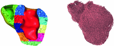
The patient-specific anatomical model was produced by using the segmentation of the end-systolic MR frame. The resulting surface mesh was further processed using the Yams software, and then the Ghs3D software was used to create a 3D tetrahedral mesh for a two-cavity (ventricular) model [5]. All the subsequent steps – for preparing the model and running simulations – were performed with the HeartLab software¹. First, specific regions of interest were designated on the outer surfaces to provide for adequate boundary conditions [14], then the tetrahedral elements were tagged according to the AHA regions specifications. Furthermore, fiber directions were prescribed based on a given variation of the elevation angle across the thickness of the walls, see Fig. 1.

Concerning the personalisation of the biophysical parameters, in this preliminary study we did not resort to automatic estimation methods as in [2], and limited ourselves to – mostly global – manual calibration based on the simplified model and then carried over to the complete 3D model. Nevertheless, this calibration process is quite complex and requires some progressive systematic strategy as explained in [1].

A major challenge for this type of patient lies in determining an adequate therapeutic strategy – usually by a combination of drugs and pacing device – specifically adapted to the patient in his/her current state, susceptible to quite rapid variations. Nevertheless, the actual cardiac state – e.g. as observed in the pressure-volume loop – is governed not only by the cardiac behavior coupled with the arterial response that determines the afterload, as accounted for in our above model, but also by the venous return that determines the preload. The latter is not included in our modeling components so far, as in fact we prescribed the preload. In order to account for variations in venous return as well, we use a description classically employed in cardiac physiology – valid for stationary states – that relies on total blood conservation written in the form [7]
where and respectively denote the distal arteries and venous system pressures, while and denote the corresponding global elastance parameters, and represents the total amount of blood that can fluctuate between the arterial and venous compartments. In addition, the distal flow between the arteries and veins is given by
where denotes the distal resistance. Of course, in a stationary regime this flow equals the cardiac output Q, hence we can use (1) to eliminate from (2) and obtain
namely, a linear relationship between cardiac output and venous pressure.

Compared with previous modeling trials, our calibration here was guided by clinical evidence that amyloidosis results into a stiffer passive behavior, while the slope of the end-systolic pressure-volume relationship (ESPVR) is roughly preserved – albeit shifted towards large volumes [11]. As a consequence, we increased the passive coefficients without changing the contractility parameter – compared to a normal heart – while adjusting the Frank-Starling function to operate with larger volumes, see [1] for a definition of this function. We show in Fig. 2 the resulting LV pressure, volume and flow indicators computed with the 3D model and compared with the processed data. We also show in Fig. 3 a comparison of the model boundaries with MRI in short axis view at end-systole and end-diastole. The calibrated biophysical parameters are given in Table 1, compared with those calibrated in [1] – in the same units – for a normal heart. As we immediately observe here, the main difference in these parameters concerns the passive law, for which an increase by a factor 20 or so – for the main two parameters – was found to be consistent with the data.