The idea of mapping measurements of blood flow onto a magnetic resonance (MR) image was first discussed in an article by Singer in 1978. The methods that followed could generally be categorized into time-of-flight (TOF) or phase shift types and were based on the techniques that had previously been described for nonimaging MR flow studies. A number of review articles have covered the subject and described the variety of methods that have been used and validated both in vitro and in vivo. The interest in flow in MR imaging has not been solely directed toward the goal of quantitative flow measurement. A large amount of effort has also been devoted to understanding the appearance of a flowing fluid on an image because this can often be indicative of the type of flow present and therefore can give important information on the diagnosis of a particular disorder. Also, the development of MR angiography techniques has required a full understanding of these effects.
In 1984, soon after the development of the first clinical MR scanners, there was an increase in interest in the search for an MR method of imaging flow. Review articles were published and a number of techniques described. This chapter provides a description and brief historical overview of the methods that have been used to measure blood flow in the heart and great vessels.
Time-of-Flight Methods
There are two categories of TOF techniques. The first, often known as wash-in/wash-out, or flow enhancement, normally rely on the saturation or partial saturation of material in a selected slice or volume being replaced by fully magnetized “high signal” spins as a result of flow ( Fig. 6.1A ). The second involves some form of tagging and then imaging to follow the motion of the tagged material ( Fig. 6.1B ).

Singer and Crooks adopted the first approach in an attempt to measure flow in the internal jugular veins, although quantification was questionable because of other factors affecting the flow signal. The first report to describe a tagged TOF approach was by Feinberg and colleagues. Their method involved a variation on a dual echo spin echo sequence; the first 180-degree selected slice was displaced by 3 mm from the initial excitation slice, and the second was displaced by 9 mm. The first 180-degree selection overlapped sufficiently with the 90-degree selection to produce a good anatomic image. The second 180-degree pulse selection did not overlap with the 90-degree or the first 180-degree pulse selection and therefore produced no anatomic image but gave high signal from the blood that had experienced all of the preceding radiofrequency (RF) pulses (i.e., that had passed between the different selected planes). The technique was used to identify flow in the carotid and vertebral arteries of a volunteer’s neck, although flow velocities had to be within a specific range and could not be defined accurately.
Methods have also been described in which the TOF flow movement can be visualized directly on an image. The methods involved the application of slice selection and frequency encoding in the same axis. In this way, material that had moved in this axis between selection and readout would be displaced relative to the stationary material. These techniques were therefore making use of signal misregistration, an effect that is often seen as a problem in other methods of flow imaging. Another TOF approach is to saturate a band of tissue, for example, in a transverse plane, and then to follow the progress of this dark band in the coronal or sagittal plane. The major limitation of these saturation methods is that they are limited by the T1 of the various tissues being saturated. The contrast of the saturated blood will decrease with time, eventually making it difficult to measure accurately the distances traveled. Also, motion during the sampling gradients results in signal and thus image distortion. In addition, for arterial flow measurements in which cardiac gating is required, only two-dimensional (2D) images can be acquired in a reasonable time so that only limited details of the flow profile can be studied.
Phase Flow Imaging Methods
Considerable knowledge had been gained on the measurement of flow from the phase of the cardiac magnetic resonance signal from the nonimaging studies after an original suggestion by Hahn in 1960 of a method of measuring the slow flow of currents in the sea. In 1984, the first attempts of measuring blood flow were described by van Dijk and Bryant and associates, using methods based on the theory suggested by Moran 2 years earlier. The imaging methods that followed fell broadly into two categories:
- 1.
Phase contrast velocity mapping methods that mapped the phase of the signal directly to measure the flow.
- 2.
Fourier flow imaging methods that phase encoded flow velocity to produce an image after Fourier transformation with velocity resolved on one image axis.
Both of these methods rely on the same principles that cause flowing material to attain a phase shift that is related to its motion. Fig. 6.2 shows these principles for a fluid flowing down a tube surrounded by stationary material. A bipolar gradient pulse is applied, consisting of a positive magnetic field gradient, followed a certain time later by an equal but opposite negative magnetic field gradient in the direction of the flow. During the period of the positive gradient, flowing and stationary materials in a particular location will take up a frequency shift that depends on their position in the direction of the field gradient. When the gradient is turned off, the phase of the flowing and stationary materials can be considered equal. In the period between the positive and negative gradients, the flowing material moves away from its stationary neighbor. During the period of the negative gradient, the stationary material takes up an equal but opposite frequency shift and returns to the phase it had before the first gradient. However, the flowing fluid takes up a different frequency shift that is dependent on the distance it has moved; its final phase therefore also depends on this distance and hence its velocity.

The relationship between the phase of the signal and flow velocity is:
ϕ=γvΔAg
The two principal approaches of using the phase shift to produce a quantitative flow image, phase contrast velocity mapping and Fourier flow imaging, are discussed in this chapter.
Phase Contrast Velocity Mapping
The early phase contrast velocity mapping methods used a spin echo sequence, which was not ideal because of problems in repeating the sequence rapidly, and signal loss as a result of shear and other more complex flows. These problems were reduced and the methods were made clinically more useful, partly by the use of a gradient echo sequence and, more importantly, by the introduction of velocity-compensated gradient waveforms.
Normally, two images are acquired with different gradient waveforms in the direction of desired flow measurement. The difference in the waveforms is calculated to produce a well-defined velocity-related phase difference between the two images. A phase reconstruction is produced for each of the images, which are then subtracted pixel by pixel to produce the final velocity map. This process of subtraction removes any phase variations that are not related to flow. The velocity phase sensitivity of the final image is normally set such that the expected velocity-related phase shifts are within the range of ± π radians. If a larger range of velocities is present, then aliasing or wrap-around will occur, resulting in measurement of ambiguous velocities. This problem can be avoided by reducing the velocity sensitivity or potentially can be corrected by a process known as phase unwrapping (described later).
Fig. 6.3A shows the phase velocity images of a series of time frames from a slice just above the heart. Flow can be seen in the ascending and descending aortas, pulmonary artery, and superior vena cava. Flow versus time curves throughout the cardiac cycle are shown in Fig. 6.3B . The stroke volume can be measured by integrating under the aortic or pulmonary flow curve. The technique has been validated both in vitro and in vivo and is now routinely used to provide useful measurements in clinical and physiologic flow studies.

Fourier Flow Imaging
Fourier flow imaging normally involves the addition of a bipolar velocity phase-encoding gradient that is stepped through a range of defined amplitudes ( Fig. 6.4 ). Because this increases the scan time by a multiple of the number of steps, it is often applied as a replacement of one of the spatial phase-encoding gradients. The image is normally reconstructed and displayed with velocity information in one dimension. Stationary material is positioned in the center of the image, with faster velocities toward the edge.

The method was first described by Redpath and colleagues in 1984; in this case, eight velocity phase-encoding steps were added to a 2D imaging sequence, to image velocities in a circle of fluid-filled tubing that rotated in the image plane. Different segments of the circle, each corresponding to different velocity ranges, were seen on the eight resultant images. A year later, Feinberg and coworkers applied the method, both in vitro and in vivo, and increased the velocity range and resolution by increasing the number of flow phase-encoding steps. In this case, however, to maintain a tolerable scan time, only one spatial phase-encoding direction was used so that there was only spatial resolution in one direction. The accuracy of the method was shown with a phantom, whereas the in vivo study, which showed the flow in the descending aorta, highlighted the problem of very high zero velocity signal from the large amount of stationary tissue imaged. In 1988, Hennig and colleagues described a development of this method in which the signal from stationary tissue was saturated and the sequence was repeated much more rapidly. The issue of time precluding the use of spatial phase encoding remains a problem, although 2D RF pulses have been used successfully to locate signals within a column. More recently, Luk Pat and associates showed a method of real-time Fourier velocity imaging that used an excited column to localize the signals. In vivo aortic flow waveforms were presented with a temporal resolution of only 33 ms.
Improving the Accuracy of Phase Contrast Velocity Measurements
The vast majority of MR flow imaging applications have used the method of phase contrast velocity mapping. The accuracy of this method is highly dependent on such factors as flow pulsatility, velocity, and size and tortuosity of the vessel. One simple approach to improving the overall accuracy of the method is to adjust the velocity sensitivity of the sequence so that the velocity-related phase shift is close to 2π for the maximum expected velocity. Buonocore extended this approach by varying the velocity sensitivity during the cardiac cycle, based on the knowledge that the arterial flow velocity is high in systole but low in diastole. The accuracy can be improved further by allowing a velocity-related phase shift greater than 2π that will result in aliasing that can be corrected by use of a phase unwrapping algorithm ( Fig. 6.5 ).

Another approach to improving accuracy has been suggested by Bittoun and associates. The method is a combination of phase contrast velocity mapping and Fourier velocity imaging with a small number of velocity phase-encoding steps. The final phase contrast velocity map is calculated from the best fit through the Fourier velocity encoded result. One potential problem with this method that can also affect conventional phase contrast velocity imaging occurs if there is any beat-to-beat variation in flow velocity. As a result of the high-velocity phase sensitivity used with this method, significant phase variations can occur, with resulting ghosting artifacts and loss of flow information.
Another method that was originally described to give a measure of velocity and flow quantification was phase contrast angiography. This technique again involves acquiring two image datasets with sequences having opposite phase velocity sensitivities, although in this case, the raw data are subtracted before reconstruction. This technique has the advantage of subtracting out signal from stationary tissue, which removes errors caused by partial volumes where voxels contained a mixture of flowing and stationary tissue. The method is, however, generally less accurate because the signal and hence the velocity measurement can be affected by factors such as in-flow enhancement and intravoxel dephasing (signal loss). In the mid-1990s, Polzin and colleagues suggested combining this method with phase contrast velocity mapping, which they showed to be more accurate in a number of phantom studies. The methods are yet to be fully validated in vivo, however, and are likely to be affected by problems of signal loss and motion, particularly when imaging is performed on small mobile vessels, such as the coronary arteries.
One of the most significant factors affecting the accuracy of the flow measurement methods is flow-related signal loss. This is normally the result of loss of phase coherence within a voxel, and eventually it results in an inability to detect the encoded phase of the flow signal above the random phase of the background noise. Even if a velocity-compensated imaging sequence is used, the acceleration and even the higher orders of motion present in complex flows can result in loss of phase coherence. Fig. 6.6 shows an example of a long-axis image of a patient with a mitral valve stenosis in which the valve is also regurgitant. In this case, a region of blood signal is lost from the ventricle during diastole as a result of the stenosis generating complex flows and from the atrium during systole because of a regurgitant jet of flow through the valve. Partial signal loss, however, does not greatly affect the accuracy of the phase contrast velocity mapping measurement unless it is accompanied by partial volume errors. When signal loss is the result of a spread of phase within a voxel, the mean phase will be detected, although this will be affected by differential saturation effects. The phase contrast velocity mapping techniques are most susceptible to signal loss of one form or another, although this can normally be minimized by appropriate gradient profile design. A good way to reduce signal loss is to use a symmetrical gradient waveform that nullifies phase shifts caused by all of the odd-order derivatives of position and then to shorten the sequence as much as possible to reduce the effects of the even-order derivatives. Signal loss of the type described is much less of a problem with the Fourier flow imaging method. In this case, the Fourier transform is used to separate out constituent velocities.

Errors can be caused by phase differences for reasons other than the velocity encoding pulses, resulting in the phase map velocity values being offset from zero, even for stationary tissues. This background phase offset generally varies gradually with position across the image, and it also varies with image plane orientation and other sequence parameters that affect the gradient waveforms, such as V enc . Distortion of the requested magnetic field gradients is unavoidable because of the fundamental laws of electromagnetism, and these are known in MR imaging as Maxwell, or concomitant, gradients. These background phase shifts become more significant when high-amplitude gradients are used and also when imaging is performed at lower main magnetic field strengths. However, with the latest gradient systems, Maxwell gradient effects are certainly a factor for phase velocity mapping at 1.5 T. However, these velocity map offsets can be corrected precisely and automatically in software, with no user intervention required. A second common reason for background phase shifts is the presence of small uncorrected side effects of the gradient pulses in the magnet, known as eddy currents. These phase shifts became more of a problem with the advent of higher-performance gradients, although more recently the problem appears to have been reduced. Software is sometimes provided that allows the user to place markers identifying stationary tissues so that this background phase error can be calculated and removed from the entire image. Sometimes, however, if the phase shifts are nonlinear or if there is little signal from stationary tissue, then the only way to correct for them is to acquire an additional set of images of a large static phantom using the same sequence parameters as those used in vivo, and then to subtract out the phase errors on a pixel-by-pixel basis.
Pixels without any signal in velocity maps have a random phase or show the phase of a weak ghost that may not be visible on the magnitude image with normal brightness settings. Particularly for poststenotic jet images, it is important to check that the magnitude image pixels of the jet are not affected by signal loss. Avoiding the inclusion of noise pixels can be problematic in regions of interest around the great vessels, and ideally, the image analysis software enables the user to set the velocity to zero for pixels whose magnitude is below a user-defined threshold.
Provided that the sequence parameters are carefully chosen such that the potential errors and artifacts discussed earlier can be minimized or avoided, phase velocity mapping has been shown to be accurate and reproducible. Validation has been reported in phantoms by comparison with true measured flow and with Doppler in animal models by comparison with in vivo flow meter measurements. Validation has also been reported in humans by comparison with methods such as Doppler ultrasound or catheterization. Perhaps the most convincing forms of validation were those performed initially by comparing the aortic flow with the left ventricular stroke volume and later flow in both the aorta and pulmonary artery with left and right ventricular stroke volumes in normal subjects. For the latter, the four measurements should be the same except for small differences caused by coronary and bronchial flow, and it can be calculated that flow measurements in large vessels are accurate to within 6%.
The effect of breath-holding on flow measurement is another factor that could affect more recent studies. Sakuma and associates showed a significant change in both pulmonary and aortic cardiac output during a large lung volume breath-hold. Conversely, flows measured during a small volume breath-hold were found to be similar to those measured during normal breathing.
There are other potential sources of error that have been reported. These include misalignment of the vessel with the direction of velocity encoding and misregistration of flow signal caused by flow between excitation and readout. Because of these and the other sources of errors discussed earlier, care is required when setting up the scan parameters, to minimize their effect.
Rapid Phase Flow Imaging Methods
With the very rapid scanning hardware available today, it is possible to repeat a phase contrast velocity sequence so fast that low-resolution images can be acquired in 100 ms or high-resolution images can be acquired in a breath-hold. The major problem is for pulsatile flow where the accuracy of the measurements and the temporal resolution can be limited if the acquisition period per cardiac cycle is too long. Also, if high spatial resolution is required, the cardiac motion of structures, such as coronary arteries, can cause blurring, with subsequent errors in flow measurement. For this reason, it is likely that more efficient k -space coverage methods, such as interleaved spirals, will be important.
Ultra-fast flow imaging techniques have also been developed, either by combining a phase-mapping type approach with imaging methods, such as single-shot echo planar and spiral imaging, or by imaging only one spatial dimension. A compromise generally has to be made in temporal or spatial resolution and probably also in the signal-to-noise ratio. However, taking into account these constraints, the methods have generally been shown to be accurate. One complication with the echo planar sequence is flow signal loss because of its inherent phase sensitivity, even when additional flow compensation is applied. However, this has been used to advantage for more qualitative flow imaging showing flow disturbances, for example.
The one-dimensional rapid acquisition mode, real-time acquisition and velocity evaluation (RACE), can be used to measure flow perpendicular to the slice. The technique can be repeated rapidly throughout the cardiac cycle to give near-real-time flow information. One problem with this type of approach is that data are acquired from a projection through the patient; this means that any signal overlapping with the flow signal will combine and introduce errors to flow measurement. Several strategies have been suggested for localizing the signal to avoid this: they include spatial presaturation, projection dephasing (applying a gradient to suppress stationary tissue), and collecting a cylinder of data and multiple oblique measurements.
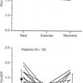
Yang and colleagues used a 2D RF excitation scheme to excite a narrow rectangular X-section column and used only 16 echoes to spatially resolve the other dimension in high resolution. This approach allowed real-time flow measurements to be acquired. The authors used the method to show the effect of controlled breathing on flow in the ascending aorta and superior vena cava ( Fig. 6.7 ).

Visualizing Flow and Flow Parameters
The method used to visualize MR flow data has depended on the method used for acquisition. For Fourier velocity measurement, each voxel may contain a range of measured velocities, and the Fourier velocity image normally takes the form of a plot of velocity versus time or velocity versus position in one direction. Fig. 6.8 shows an example in which velocity images were acquired from a column of excited tissue, including the descending aorta. The front edge of the aortic pulse wave can be seen on successive frames as it travels down the vessel.

Phase contrast velocity images contain only one velocity measure per image voxel. Historically, these have been shown with a gray scale such that flow in one direction tends toward white, flow in the other direction tends toward black, and stationary material is mid-gray, as shown previously in Fig. 6.3A . When flow is measured in more than one direction, more sophisticated methods of display can be used. Fig. 6.9 shows a vector map of flow in the root of the aorta of a patient with an atherosclerotic aneurysm. This systolic image, shown alongside a pressure map (described later), shows high-velocity flow impinging on the wall of the aneurysm. An alternative type of representation would be to use the cine velocity images to calculate the path of a seed over time.