Data Acquisition and Corrections

(1)

Cleveland Clinic, Emeritus Staff, Cleveland, OH, USA

Keywords

PET dataSinogramPET/CTPET/MRAttenuation correctionTime of flightArtifacts

PET Data Acquisition

Positron emission tomography (PET) is based on the detection in coincidence of the two 511-keV annihilation photons that originate from β ⁺ emitting sources (e.g., the patient). The two photons are detected within an electronic time window (e.g., 12 ns) set for the scanner and must be along the straight line connecting the centers of the two detectors called the line of response (LOR). Since the two photons are detected in coincidence along the straight line in the absence of an absorptive collimator, this technique is called electronic collimation. All coincident events are collectively called prompts, which include true, random, scattered, and multicoincidence events. Examples of these events are illustrated in Fig. 3.1. A true coincident event arises when two 511-keV photons from a single annihilation event are detected by a detector pair along the LOR within the set energy and timing window (Fig. 3.1a). Random coincidences occur when two unrelated 511-keV photons from two separate annihilation events are detected by a detector pair within the same time window (Fig. 3.1b). These events raise the background in the image causing loss of image contrast. Scatter coincidences occur due to Compton scattering of annihilation photons in the patient, and one 511-keV photon and one scattered photon or both scattered photons arising from the same annihilation event may fall within the 511-keV energy window and be detected by a detector pair within the coincidence time window (Fig. 3.1c). Note that two scattered photons from two separate annihilation events falling within the set energy and timing windows will be counted as a random coincident event. Scatter coincidences raise the background of the image and degrades the image contrast. Multicoincidence occurs when more than two unrelated 511-keV photons are detected in coincidence in different detectors within the time window, but these events are discarded because of the difficulty in positioning them. The detailed description of different coincident events is given later.

Fig. 3.1

(a) True coincident events that result from two 511-keV photons from a single annihilation event and detected along an LOR by a detector pair within the set energy and timing windows. (b) Random coincidences occur when photons from two unrelated annihilation events are detected by a detector pair along the LOR (dotted line). (c) Scattered coincident events result when one or both 511 keV photons from a single annihilation are scattered in the body tissue and one scattered photon and the unscattered 511 keV photon, or both scattered photons, are detected by a pair of detectors along the LOR within the set energy and timing windows

In a full ring system, the data are collected simultaneously by all detector pairs, whereas in partial ring systems, the detector assembly is rotated around the patient in angular increments to collect the data. In acquiring the coincidence events, three steps are followed:

The location of the detector pair in the detector ring is determined for each coincident event.

The pulse height of the photon detected is checked if it is within the energy window set on 511 keV.

Finally, the position of the LOR is determined in terms of polar coordinates to store the event in the computer memory.

As stated in Chap. 2, in a PET scanner, block detectors are cut into small detectors and coupled with four PM tubes, which are arranged in arrays of rings. Each detector is connected in coincidence to as many as N/2 detectors, where N is the number of small detectors in the ring. So which two detectors detected a coincidence event within the time window must be determined. Pulses produced in PM tubes are used to determine the locations of the two detectors (Fig. 3.2). As in scintillation cameras, the position of each detector is estimated by a weighted centroid algorithm. This algorithm estimates a weighted sum of individual PM tube pulses, which are then normalized with the total pulse obtained from all PM tubes. Similar to scintillation camera logistics, the X and Y positions of the detector element in the ring are obtained as follows:

Fig. 3.2

A schematic block detector is segmented into 8 × 8 elements, and four PM tubes are coupled to the back of the block for pulse formation. The pulses from the four PM tubes (A, B, C, and D signals) determine the location of the element in which 511-keV γ-ray interaction occurs, provided the sum of the four pulses falls within the energy window of 511 keV

$X=\frac{\left(B+C\right)-\left(A+D\right)}{A+B+C+D},$

(3.1)

$Y=\frac{\left(C+D\right)-\left(A+B\right)}{A+B+C+D}.$

(3.2)

Here A, B, C, and D are the pulses from the four PM tubes as shown in Fig. 3.2.

The four pulses (A, B, C, D) from four PM tubes are then summed up to give a Z pulse, which is checked by the pulse height analyzer (PHA) if its pulse height is within the energy window set for the 511-keV photons. If it is outside the window, it is rejected; otherwise, it is accepted and processed further for storage.

The last step in data acquisition is the storage of the data in the computer. Unlike conventional planar imaging where individual events are stored in an (X, Y) matrix, the coincidence events in PET systems are stored in the form of a sinogram. Consider an annihilation event occurring at the ∗ position in Fig. 3.3a. The coincidence event is detected along the LOR indicated by the arrow between the two detectors. It is not known where along the line of travel of the two photons the event occurred, since photons are accepted within the set time window (say, 12 ns) and their exact times of arrival are not compared. The only information we have is the positions of the two detectors in the ring that registered the event, i.e., the location of the LOR is established by the (X, Y) positioning of the two detectors. Many coincidence events arise from different locations along the LOR and all are detected by the same detector pair and stored in the same pixel.

Fig. 3.3

PET data acquisition in the form of a sinogram. Each LOR data is plotted in (r,ϕ) coordinates (a). Data for all r and ϕ values are plotted to yield the sinogram indicated by the shaded area (b). (Only a part of the sinogram is shown.) (Reprinted with the permission of the Cleveland Clinic Center for Medical Art and Photography ^©2009. All rights reserved)

For data storage in sinograms, each LOR is defined by the distance (r) of the LOR from the center of the scan field (i.e., the center of the gantry) and the angle of orientation (ϕ) of the LOR (i.e., the angle between r and the vertical axis of the field). If we plot the distance r on the x-axis and the angle ϕ on the y-axis, then the coincidence event along the LOR (r, ϕ) will be assigned at the cross-point of r and ϕ values (Fig. 3.3b). In a given projection, adjacent detector pairs constitute parallel LORs (at different r values in Fig. 3.3a) at the same angle of orientation. The plot of these LORs will be seen as a horizontal row at angle ϕ. When all projections around the field of view are obtained, the plot of the LORs at different projection angles and r values will result in the shaded area shown in Fig. 3.3b, which is called a sinogram. A sinogram is essentially a matrix of fan-beam projections defined by the angle of acceptance. A typical normal sinogram is shown in Fig. 3.4.

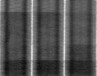
Fig. 3.4

A typical normal sinogram indicating all detectors are working properly

PET data are acquired directly into a sinogram in a matrix of appropriate size in the computer memory. The sinogram is basically a two-dimensional (2D) histogram of the LORs in the (distance, angle) coordinates in a given plane. Thus, each LOR (and hence, detector pair) corresponds to a particular pixel (or element) in the sinogram, characterized by the coordinates r and ϕ. For each coincidence event detection, the LOR is determined, the corresponding pixel in the sinogram is located, and a count is added to the pixel. In the final sinogram, the total counts in each pixel represent the number of coincidence events detected during the counting time by the two detectors along an LOR.

It is of note that comparing raw data acquired in PET with those in SPECT, each projection image in SPECT represents data acquired at that projection angle across all slices, whereas in PET, each sinogram represents the data acquired for a slice across all angles. A set of sinograms from a complete, multislice PET study can be deciphered in the computer to generate a series of projection views that are similar to SPECT raw data.

Data are acquired in either frame mode or list mode. Details of these acquisitions are given in books on physics in nuclear medicine, and the readers are referred to them. Briefly, in frame mode, digitized signals are collected and stored in X, Y positions in a matrix of given size and depth for a specified time or total number of counts. In list mode, digitized X– and Y-signals are coded with “time marks” as they are received in sequence and stored as individual events as they occur. After the acquisition is completed, data are manipulated to form images in a variety of ways to meet a specific need. This process is time consuming despite the wide flexibility it provides. In PET studies, while the frame mode acquisition is routinely used, with the introduction of faster computers, the list mode acquisition is now being used more commonly for the newer cameras.

Data can be acquired in both static and dynamic imaging using either list mode or frame mode. In static imaging, a single-frame image is acquired by collecting data over a period of time normally in frame mode. In dynamic imaging, data are collected in multiple frames of sinograms, each of a predetermined period of duration. An example of dynamic imaging is cardiac blood pool gated studies in which the duration of the cardiac QRS cycle is deciphered into nearly 20-ms time segments and list mode data are acquired sequentially for each segment. Acquisition is repeated for many QRS cycles for the data to be statistically meaningful. List mode data are then binned into sinograms and sequential frame mode images are obtained. Whereas static images provide an estimate of gross tracer uptake, dynamic imaging provides the kinetics of tracer uptake in an organ.

How many counts need to be acquired per projection and what size matrix should be chosen for adequate quality of images vary with the different cameras depending on the scatter, random, and extent of smoothing needed. A three-dimensional (3D) scanner would acquire more counts per projection than a 2D scanner because of the more scatter events in the 3D scanner. Typically 250,000–500,000 counts are needed for optimal quality of images. For good-quality images, the pixel size is recommended to be 2–3 mm. If the FOV is of the order of 300 mm acquired in a128 × 128 matrix, then pixel size would be ~2.3 mm indicating the right choice of the matrix for data acquisition.

Since PET systems are axially fixed, whole-body imaging is accomplished by moving a computer-controlled bed with the patient on it along the axial field and collecting data at adjacent bed positions. In whole-body imaging, the total scan time depends on the patient’s body length and the effective axial FOV of the scanner per bed position. Since the sensitivity decreases toward the periphery of the FOV, the effective axial FOV is less than the actual FOV and it is necessary to overlap the bed positions in whole-body imaging. A typical overlap of 3–5 cm is common, and an even higher value is used in 3D acquisition, because of the sharper decrease in sensitivity toward the periphery of the FOV. The time for data acquisition at each bed position in whole-body imaging is 5–10 min.

Time-of-Flight Method

The time-of-flight (TOF) PET technique is based on the measurement of time difference in the arrival of the two 511-keV annihilation photons at the detectors, as illustrated in Fig. 3.5. Suppose two detectors are equidistant, x, from the center of FOV (CFOV) and a positron is annihilated in the patient at position ∗ at a distance Δx from the CFOV. One of the 511-keV photons will travel x + Δx in time t ₁ and the other will travel x − Δx in time t ₂. Since the photons travel at the speed of light (c), the difference in time of arrival (Δt = t ₁ − t ₂) of the two photons at the detectors is 2Δx/c. Note that the photons from the CFOV arrive at the detectors simultaneously (Δx = 0). The value of x is known but the location of positron annihilation on the LOR is not known. It is determined by the uncertainty in the point of interaction given by Δx = (c · Δt)/2. From the knowledge of the time difference Δt of the photon arrival, Δx is calculated, which is the distance along the LOR away from the midpoint between the two detectors to where the annihilation took place. This localization information is then stored in the computer matrix for image reconstruction later. With faster electronics and improved scintillators, and also shorter time windows, it is possible to measure the time difference Δt fairly accurately by TOF PET scanner and thus to determine the accurate location of the annihilation event providing high-resolution images.

Fig. 3.5

A schematic diagram illustrating the principle of time-of-flight (TOF) technique. The time difference (t ₁ − t ₂) in the arrival of two photons is related to the difference in distances Δx, traveled by them. Using TOF information, the annihilation point is determined within a spatial range of Δx = (c · Δt)/2, which is stored in the matrix to generate images (Reprinted with the permission of the Cleveland Clinic Center for Medical Art and Photography ^©2009. All rights reserved)

The parameter Δx is usually much smaller than the diameter D of the patient (with good timing resolution). The signal-to-noise ratio (SNR) or sensitivity increases with improved timing resolution and is proportional to D/Δx, i.e., 2D/(c · Δt). For a 30-cm subject and a timing resolution of 0.5 ns, the SNR (sensitivity) increases by a factor of 4.

Decades ago, the TOF PET scanners were introduced using fast detector like cesium fluoride (CsF) or barium fluoride (BaF₂) to allow high count rates, but spatial resolution and sensitivity were poorer than those of conventional PET scanners with BGO, because of poor light production. With the advent of improved scintillators like LSO, LYSO, and LaBr₃, along with more efficient and reliable PM tubes, TOF is currently adopted in several conventional commercial PET scanners. Philips Healthcare is marketing Big Bore Gemini TF PET scanners based on the TOF technique. Current TOF scanners offer better spatial resolution and sensitivity because of increased light production in the detector material and the shorter timing resolution. Moreover, this technique improves the image quality in heavy patients, compared to the PET scanners that lead to a loss of counts due to attenuation as well as an increase in scattered counts.

Two-Dimensional vs. Three-Dimensional Data Acquisition

Coincidence events detected by two detectors within the time window are termed “prompt” events. The prompts include true, random, and scatter coincidence events. In many PET systems, in an attempt to eliminate random and scatter photons discussed later, annular septa (~1-mm thick and radial width of 7–10 cm) made of tungsten or lead are inserted between rings (Fig. 3.6a). In some scanners, septa are retractable or fixed, while in others, they are not incorporated, depending on the manufacturers. These septa function like the parallel-hole collimators in scintillation camera imaging. Only direct coincidence events between the two paired detectors in a ring are recorded. Such counting is called the 2D mode of data acquisition. In this mode, most of the random and scattered photons from outside the ring are prevented by the septa to reach the detectors, leaving the true coincidences to be recorded (Fig. 3.6a). The use of septa reduces the fraction of scattered photons from 30 to 40% without septa to 10–15%.

Fig. 3.6

(a) 2D data acquisition with the septa placed between the rings so that true coincidence counts are obtained avoiding randoms and scatters. Detectors connected in the same ring give direct plane events. However, detectors are connected in adjacent rings and cross plane data are obtained as shown. (b) When septa are removed, the 3D data acquisition takes place, which include random and scatter events along with true events

Detector pairs connected in coincidence in the same ring give the direct plane event (Fig. 3.6a). To improve sensitivity in 2D acquisition, detector pairs in two adjacent rings are connected in coincidence circuit. Coincidence events from a detector pair in this arrangement are detected and averaged and positioned on the so-called cross plane that falls midway between two adjacent detector rings (Fig. 3.6a). In current PET scanners, small detectors are used for better resolution but result in low sensitivity in the direct and cross planes. So additional cross planes are included from nearby rings that are connected in coincidence so that the overall sensitivity of the scanner is increased. The acceptable maximum number of rings that are connected in coincidence for cross planes is 5 or 6. Note that for an n-ring system, n direct planes and n − 1 cross planes can be obtained in 2D acquisition. Thus, a total of 2n − 1 sinograms are generated, each of which produces a transaxial image slice. While the cross planes increase the sensitivity, they degrade the spatial resolution.

The overall sensitivity of PET scanners in 2D acquisition is 2–3% at best. To increase the sensitivity of a scanner, the 3D acquisition has been introduced in which the septa are retracted or they are not present in the scanner (Fig. 3.6b). This mode includes all coincidence events from all detector pairs, thus increasing the sensitivity by a factor of almost 4–8 over 2D acquisitions. If there are n rings in the PET scanner, all ring combinations are accepted and so n ² sinograms are obtained. However, scattered and random coincidences are increasingly added to the 3D data, thus degrading the spatial resolution as well as requiring more computer memory. As a trade-off, one can limit the angle of acceptance to cut off the random and scattered radiations at the cost of sensitivity. This can be achieved by connecting in coincidence each detector to a fewer number of opposite detectors than N/2 detectors. The sensitivity in 3D mode is highest at the axial center of the field of view and gradually falls off toward the periphery. Three-dimensional data require more storage as they are approximately 10³ times more than 2D data and so result in time-consuming computation. However, current fast computers have significantly overcome this problem.

Factors Affecting Acquired PET Data

The projection data acquired in the form of sinograms are affected by a number of factors, namely, variations in detector efficiencies between detector pairs, random coincidences, scattered coincidences, photon attenuation, dead time, and depth of interaction. Each of these factors contributes to the sinogram to a varying degree depending on 2D or 3D acquisition and needs to be corrected for prior to image reconstruction. These factors and their correction methods are described below.

Normalization

Current PET scanners can have 10,000–35,000 detectors arranged in blocks and coupled to several hundred PM tubes. Because of the variations in the gain of PM tubes, the location of the detector in the block, and the physical variation of the detector, the detection efficiency of a detector pair varies from pair to pair, resulting in nonuniformity of the raw data. This effect in dedicated PET systems is similar to that encountered in conventional scintillation cameras used for SPECT and PET studies. The method of correction for this effect is termed the normalization. Normalization of the acquired data is accomplished by exposing uniformly all detector pairs to a 511-keV photon source (e.g., ⁶⁸Ge source), without a subject in the field of view. Data are collected for all detector pairs in both 2D and 3D modes, and normalization factors are calculated for each pair by dividing the average of counts of all detector pairs (LORs) by the individual detector pair count. Thus, the normalization factor F _ifor each LOR is calculated as

${F}_i=\frac{A_{\mathrm{mean}}}{A_i},$

(3.3)

where A _mean is the average coincidence counts for all LORs in the plane and A _iis the counts in the ith LOR. The normalization factor is then applied to each detector pair data in the acquisition sinogram of the patient as follows:

${C}_{\mathrm{norm},i}={C}_i\times {F}_i,$

(3.4)

where C _iis the measured counts and C _norm,iis the normalized counts in the ith LOR in the patient scan. A problem with this method is the long hours (~6 h) of counting required for meaningful statistical accuracy of the counts, and hence overnight counting is carried out. These normalization factors are generated weekly or monthly. Most vendors offer software for routine determination of normalization factors for PET scanners. A difficulty with this method is that scatter and random coincidences require different normalizations from true coincidences, which is difficult to accomplish separately.

A component-based variance reduction method is employed to partially resolve these problems. Normalization factors are calculated as the product of intrinsic crystal efficiencies and geometric factors that account for the variation in crystal efficiency with the position of the crystal in the block and photon incidence angle. Intrinsic efficiencies of individual detectors are determined from the average sum of the coincidence efficiencies between a given detector and all opposite detectors connected in coincidence. The geometric factors are normally determined by the manufacturers using a very high activity source and they presumably remain constant. This reduces the computation from the number of LORs (millions) to the number of detectors (thousands). Even though normalization by the component-based method is less time consuming, residual artifacts in images reconstructed from normalized acquisitions of uniform phantoms have been reported.

Photon Attenuation

Attenuation of annihilation photons occurs due to their absorption and scattering in the body tissue. The extent of attenuation depends on the depth of tissue the photons have to travel before striking the detector. Photons in the center of the body undergo maximum attenuation, because they travel the most depth of the tissue, whereas those at the periphery are least attenuated. Attenuation also occurs when annihilation photons traverse across different organs or tissues. This causes uneven distribution of counts over regions of interest. Therefore, attenuation correction must be applied to the acquired data prior to image reconstruction.

If μ is the linear attenuation coefficient of 511-keV photons in the tissue, and a and b are the tissue thicknesses traversed by the two 511-keV photons along the LOR (Fig. 3.7), then the probability P of coincidence detection is given by

Fig. 3.7

Two 511-keV photons detected by two detectors suffer attenuation after traversing two different tissue thicknesses, a and b. D is equal to the sum of a and b. Attenuation of 511-keV photons is independent of the location of annihilation and depends on the total dimension of the body as given by Eq. (3.5) (Reprinted with the permission of the Cleveland Clinic Center for Medical Art and Photography ^©2009. All rights reserved)

$P={\mathrm{e}}^{-\mu a}\times {\mathrm{e}}^{-\mu b}={\mathrm{e}}^{-\mu \left(a+b\right)}={\mathrm{e}}^{-\mu D},$

(3.5)

where D is the total thickness of the body. Equation (3.5) is applicable to organs or tissues of uniform density. All coincident events along the same LOR will have the attenuation effect given by Eq. (3.5). When photons travel through different organs or tissues with different μ values, then Eq. (3.5) becomes

$P={\mathrm{e}}^{-{\displaystyle \sum_{i=0}^n{\mu}_i{D}_i}},$

(3.6)

where μ _iand D _iare the linear attenuation coefficient and thickness of the ith organ or tissue, respectively, and n is the number of organs or tissues the photon travels through. Photon attenuation causes nonuniformities in the images (Fig. 3.8), because of the loss of relatively more coincidence events from the central tissues than from the peripheral tissues of an organ and also because the two photons may transverse different organs along the LOR.

Fig. 3.8

(a) Profile of raw acquired data showing depression in activity due to more attenuation at the center. (b) The same profile with attenuation correction (Reprinted with the permission of the Cleveland Clinic Center for Medical Art and Photography ^©2009. All rights reserved)

Note that the probability P is the attenuation correction factor, which is independent of the location of positron annihilation and depends on the total thickness of the tissue. If an external radiation passes through the body, the attenuation of the radiation will be determined by an effective attenuation coefficient μ (tissues of different μ _i) and the thickness of the body, as expressed by Eq. (3.5). This introduces the transmission method of attenuation correction, by using an external source of radiation rather than using the patient as the emission source, and the method is described below.

Attenuation Correction Methods

Theoretical Method

A simple theoretical calculation based on Eq. (3.5), also called the Chang method, can be applied for attenuation correction based on the knowledge of μ and the contour of an organ, such as the head, where uniform attenuation can be assumed. However, in organs in the thorax (e.g., heart) and the abdomen areas, attenuation is not uniform due to the prevalence of various tissue structures, and the theoretical method is difficult to apply and, therefore, a separate method such as the transmission method is employed.

Only gold members can continue reading. Log In or Register to continue