and Laurence Loeuillet2
(1)
Centre d’échographie Ambroise Paré, Les Mureaux, France
(2)
Hôpital Cochin, Paris, France
Corpus Callosum
Anatomy of the Corpus Callosum
The corpus callosum is the main commissure (bundle of neural fibers crossing the midline and connecting the two cerebral hemispheres). It is made up of four parts, from front to back: rostrum, genu, body, and splenium.


Development of the Corpus Callosum
The corpus callosum develops from front to back in a rotating movement.

Ultrasonographic Features of the Corpus Callosum
16 gw

It is possible to visualize the genu of the corpus callosum from 16 gw (yellow arrows).
17 gw


Fetal pathology specimen at 18 gw
19 gw

21 gw


Fetal pathology specimens at 20–21 gw
23 gw


Fetal pathology specimens at 22, 23, and 24 gw
23 gw Omniview

25 gw


Fetal pathology specimen at 24 gw
27 gw

Fetal pathology specimen at 27 gw
29 gw

30 gw

32 gw

32 gw

34 gw

Ideally, the corpus callosum should be visualized in a sagittal image by conventional 2D or 3D ultrasound.
Volume reconstruction from an axial plane (figure below) provides an indirect indication as to the presence of the corpus callosum: the echoic formation (yellow arrows) corresponds to the interface between the septum pellucidum and underlying tissues and vessels such as the pericallosal artery (Pilu et al. 2006; Malinger et al. 2007, 2009; Plasencia et al. 2007). This interface must not be confused with a lipoma of the corpus callosum.
The corpus callosum may nevertheless sometimes be visualized as a finely echoic band located beneath this interface (green arrow).
Coronal images are particularly useful, in particular for detecting indirect signs: abnormal orientation of the frontal horns (see agenesis of the corpus callosum). The pathway of the pericallosal artery (which is seen in a sagittal plane) will be discussed in the section on “Cerebral circulation”.

Lateral Ventricles
Lateral Ventricles: Biometrics and Images
Biometrics
The size of the lateral ventricles should be determined by measuring atrial diameter.
In order to guarantee the quality and reproducibility of such measurements, the method employed must be perfectly standardized.
Two proposals have so far been issued concerning the standardization of such measurements:

Measurements must be made at the glomus of the choroid plexus, perpendicularly to the cavity, with the calipers places “on to on.” This method calls for a few comments: the axial measurement plane would not appear to be perfectly defined as the position of the glomus may vary as it is affected by gravity.
Laurent Guibaud’s Score (Fig. 3.2)
This method has the advantage of strictly defining the plane and point at which the measurement is made. The author also provides a scoring system that can be used for quality control.
The midline must be placed horizontally with a perfectly symmetrical plane. The anterior anatomical landmark is the lower part of the septal cavity or, even better, the point at which the crura of the fornix join together (green square), i.e., very slightly below the septum. The posterior anatomical landmark is the cisterna ambiens: triangular formation with a posterior peak located slightly rearward of the thalami (pink figure). The measurement is made perpendicularly to the walls of the ventricles at the internal occipital sulcus (white arrow) (Figs. 3.2 and 3.3).


Fig. 3.2
Landmarks for Laurent Guibaud’s score
Fig. 3.3
Calipers at the appropriate localisation
Using 3D ultrasound and splitting into three planes (Fig. 3.4) can best locate the anterior anatomical landmarks on the anterior part of the crura of the fornix.

Fig. 3.4
Using 3D ultrasound and splitting into 3 planes
A score may be established using a model similar to that published by Herman to assess the quality of nuchal translucency measurements.
Criteria | Score | Technical requirements |
|---|---|---|
Axial plane only | 0–2 | Midline perpendicular to the transducer, equivalent distances from the cranial walls |
Appropriate section position | 0–1 | Anterior anatomical landmark: crura of fornix Posterior anatomical landmark: cisterna ambiens |
Measurement point | 0–1 | At the internal occipital sulcus |
Caliper position | 0–2 | Measurement made perpendicularly to the walls of the ventricles Calipers “on to on” |
Image size | 0–1 | Image of the cranium filling the entire screen with the contours of the cranium visible |
The maximum score possible is 7 (the primary criteria are underlined in red, the secondary criteria in blue). A score of more than 5 is considered to be acceptable.
It should be noted that these measurements are made only on the ventricles that are distal to the transducer. It is therefore important to check the appearance of the anterior horns. If the proximal anterior horn seems to be unusually broad, the atrial diameter of the ventricle must be measured after changing fetal position either by spontaneous movements of the fetus, gently moving the fetus, or seeing the patient again some time later.
Morphology

Fig. 3.5
Diagram of the ventricular system. CP posterior horn, CF frontal horn, CT temporal horn, V3 third ventricle, V4 fourth ventricle
This diagram illustrates the connections between the cerebral ventricles: the two lateral ventricles communicate with the third ventricle via the foramina of Monro. The third ventricle in turn communicates with the fourth ventricle via the cerebral aqueduct. Finally, the fourth ventricle communicates with the arachnoid spaces via the median aperture on the midline and via the paired lateral aperture.

Ventricular system at 40 gw (V4 °, V3 *)

Fig. 3.6
Ventricle walls and content
It is important to assess not only the size of the ventricles but also visualize their walls while examining for any hyperechoic areas and their contents while examining for echogenic structures suggestive of clots that could indicate intraventricular hemorrhage (Fig. 3.6).
Sylvian Fissure
Sylvian Fissure and Study of the Gyration
Development of the cerebral cortex is divided into three phases:
Proliferation and differentiation of neuronal precursor cells
Neuronal migration to the surface along migratory tracts to create cerebral lamination up to 20 gw (Fig. 3.7c) (Pugash 2012)
Rapid development of the superficial layer but without development of the deep layers, accompanied by synapse creation and apoptosis
Although any study of the gyration is the prerogative of MRI, which, by its technical aspects, can be used to assess the cerebral cortex in its entirety, the sonographer may, particularly by studying the Sylvian fissure and some of the main sulci, provide a useful and informative assessment of the gyration.
Sylvian Fissure
This may be studied in the axial plane, but the coronal plane is more appropriate.


Fig. 3.7
(a) Sylvian fissure in a coronal image at 22 gw, (b) shape of the Sylvian fissure at 27 gw in parasagittal images (TUI volume mode), (c) cerebral lamination: green arrows, white arrows: migratory tracts (TUI volume mode)
Fetal pathology specimens at 22 gw


Fig. 3.8
Sylvian fissure at 25 gw axial image
Fetal pathology specimens at 25 gw
Sylvian fissure operculization may be assessed by calculating a score (Quarello et al. 2008) that includes the angle formed by the base of the Sylvian fissure and the anterior edge of the insular lobe and the extent to which this edge is curved. This measurement should be made in the axial plane from the crura of the fornix at the front to the cisterna ambiens at the rear (passing through the third ventricle). The score ranges from 1 to 10. In the example below (Fig. 3.9), the score is 3, corresponding to the 50th percentile at 25 gw.
Scores for various time points are shown below: