Diffusion and Diffusion Tensor MR Imaging: Fundamentals
Peter J. Basser
Introduction
Along with the evolution and maturation of conventional magnetic resonance imaging (MRI) methods over the last three decades, it has also become apparent that the measurement of diffusion properties in neural tissue provides unique information that has demonstrated biologic and clinical relevance. Specifically, diffusion properties of tissue constituents reveal characteristics of tissue microstructure and architectural organization. Moreover, this information is obtained noninvasively and without exogenous contrast agents, solely by measuring the mobility of water in tissues. Indeed, diffusion MRI sequences are ubiquitous and are routinely implemented in clinical MRI studies evaluating cerebral tissue for the presence of disease. In a growing number of conditions affecting brain structure, more complex diffusion sequences are being used to serve as the microanatomic correlate of altered microstructure in a wide range of clinical disease states. Before looking at the specific structural and architectural features that can be inferred from MR diffusion measurements, this chapter establishes the conceptual and methodologic underpinnings of diffusion nuclear magnetic resonance (NMR) and diffusion MRI.
Physical Underpinnings of Diffusion NMR and MRI
The classic macroscopic, phenomenologic picture of molecular diffusion is best exemplified by considering the behavior of molecules within a diffusion cell (Fig. 27.1). There, molecular solutions of different concentrations placed in two initially separate compartments are allowed to mix together through a permeable membrane between them. A net macroscopic molecular flux, J, can be observed as particles move from the compartment of higher concentration to that of lower concentration. Fick’s first law, a phenomenologic relationship between J and the concentration gradient, describes this mixing process. In it, the scalar diffusion coefficient, D, appears as a scaling factor. Rapid mixing between compartments results when the diffusivity is high; slower mixing results when the diffusivity is low. A variety of tracer techniques can be used to measure diffusion coefficients from the simultaneous measurement of the flux and the concentration gradient or from concentration profiles measured as a function of time (1,2), but all such methods require either chemically or physically labeling the tracer molecules and detecting their distribution. Invasive tracer experiments have been performed to determine the diffusivity of metabolites in the brains of animals (3,4).
The discovery of Brownian motion (5) and the development of mathematical models describing it provided the basis of the modern picture of molecular diffusion (6,7). In the Brownian view, diffusion is a process that causes molecules to mix because of random collisions among the diffusing molecules (self diffusion) or because of collisions with other molecules. This conceptual picture is represented schematically in Figure 27.2 by a jagged trajectory of an individual molecule buffeted by random collisions with neighboring molecules. Unlike the deterministic picture of molecular transport implicit in Fick’s first law, the Brownian description is inherently a probabilistic one. Although the precise trajectory of each molecule is not known per se, their aggregate behavior—embodied in the displacement probability distribution—can still be determined. Specifically, the displacement distribution is the probability of finding a molecule at a particular position and at a particular time, given that it previously occupied another position at an earlier time. One of many fundamental contributions made by Einstein (7) to understanding the physics of diffusion was to relate the variance of this Brownian displacement distribution—the mean-squared displacement in one dimension, < x2>—to the diffusion coefficient, D, appearing in Fick’s first law and the diffusion time, τ:
(In three dimensions, the coefficient 2 should be replaced by 6.) Thus, the larger the diffusion coefficient, D, the greater the distance a particle is expected to travel on average during the same diffusion time.
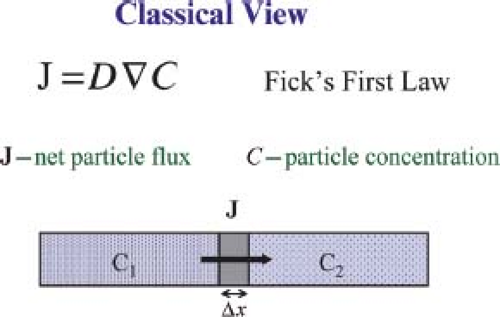 FIGURE 27.1 The Fickian picture of diffusion is best understood by considering the behavior of the diffusion cell, schematically represented here, in which the particle concentration is different in two compartments that are separated by a permeable membrane. |
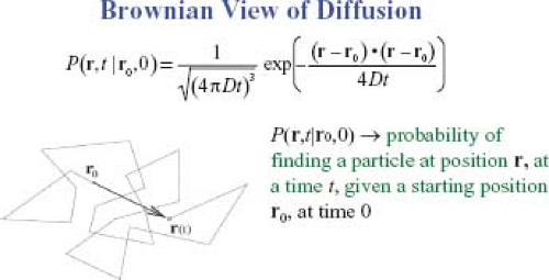 FIGURE 27.2 The Brownian picture of diffusion is best epitomized by this sketch illustrating a possible path taken by a molecule that is released at point r0 at time t = 0 and moves to position r at a later time t. The molecule undergoes a “drunken walk” whose displacement is characterized by a probability distribution. |
Classic NMR measurements of (translational) molecular diffusion were based on the Brownian rather than the Fickian picture. The distinction is important because the Brownian description enables one to measure a molecular diffusion coefficient without using exogenous tracers. In essence, in the NMR measurement of diffusion, the diffusivity is inferred from the phase dispersion of the magnetization (loss in signal) caused by the assumed random displacements of spin-labeled molecules. Moreover, the Brownian pictures can treat diffusion as a process that can occur at thermodynamic equilibrium. One no longer needs to set up concentration gradients to observe diffusion.
The first person to understand and describe the effect of molecular diffusion on the NMR signal was Erwin Hahn (8). The first measurements of the self-diffusivity of water (and of other liquids) using NMR methods were reported in the 1950s (9). In a series of classic experiments, Carr and Purcell used the NMR spin echo, also discovered by Hahn (8), to measure the self-diffusion coefficient of water and other solvents (9). Carr and Purcell first showed that the NMR spin echo could be sensitized specifically to the translational motion of a spin-labeled species by subjecting it to a static magnetic field gradient. An example of their NMR sequence is given in Figure 27.3A. They then showed that the random motions (net displacements) caused by diffusion reduce the amplitude of the NMR spin echo. The larger the diffusivity of the spin-labeled molecules, the greater the phase dispersion and the larger the attenuation of the magnitude signal they observed. By using a Brownian, probabilistic description of molecular displacements of the spin system subjected to a uniform magnetic field gradient, they derived an analytic expression relating the NMR signal attenuation and the molecular diffusion coefficient. Their conceptual framework is the basis for modern diffusion MRI studies. Their work also established the nonperturbing and highly accurate NMR measurement of the self-diffusion coefficient of water and other solvents as a “gold standard.”
Two years later, Torrey incorporated the diffusion of magnetized spins explicitly into the Bloch (magnetization transport) equations (10), showing how it leads to additional attenuation, the NMR signal (11). Analytic solutions to this equation followed for freely diffusing species during a spin-echo experiment (12) and, later, for diffusion in various restricted geometries (13,14,15), in which the diffusing species were confined within pores of varying shapes.
The next key innovation in the evolution of NMR diffusion measurements was the development and use of pulsed-field gradient methods (16). By applying two appropriately placed short-duration magnetic field gradient pulses rather than one that is constant in time, the NMR diffusion experiment could be performed more accurately and with an ability to control independently the diffusion time and length scale that is probed (14). An example of a pulsed gradient sequence is shown in Figure 27.3B. Using their new pulsed gradient sequence, Stejskal and Tanner extended the findings of Carr and Purcell, showing that uniformly translating spins produce a net phase shift that is proportional to their velocity and that diffusing spins produce no net phase shift but a change in the height of the phase distribution (16). They generalized the mathematical framework of McCall et al. (17) for relating the signal attenuation, A/A0; the conditional displacement distribution, P(r2, Δ|r1, 0); the pulse duration, δ; the pulse strength, G; the gyromagnetic ratio, γ; and the time between pulses, Δ:
where the assumption is also made that δ is infinitesimally short so that negligible molecular displacements occur during the pulse period as compared with during the diffusion time, that is, δ ≪ Δ.
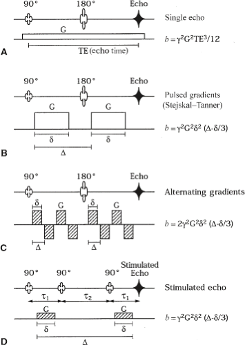 FIGURE 27.3 Several paradigmatic diffusion sequences are shown with the radiofrequency signal on the top line and the diffusion gradient pulse train on the bottom line. The corresponding b values (which measure the degree of diffusion weighting of the nuclear magnetic resonance signal) are given in terms of the gradient strength, G, pulse width, Δ, and pulse separation, Δ. Spin-echo sequences include (A) a constant gradient, (B) matched rectangular gradients, and (C) alternating gradients. A diffusion-weighted stimulated echo sequence is also shown (D). Generally, each diffusion sequence can be incorporated into virtually any magnetic resonance imaging sequence to produce a diffusion-weighted image. |
Here, P(r1,0) is the initial distribution of spins, and P(r2, Δ|r1, 0) is the probability that a particle starting at position r1 at time 0 ends up at position r2 at time Δ.
This equation looks formidable, and generally it is difficult to evaluate analytically in all but the simplest of geometries (18).
In the simplest case—free diffusion in an unbounded, isotropic, homogeneous medium—P(r2, Δ|r1, 0) is Gaussian:
In the simplest case—free diffusion in an unbounded, isotropic, homogeneous medium—P(r2, Δ|r1, 0) is Gaussian:
or
where D is the diffusion coefficient and r is the net displacement, r = r2 − r1. If we also assume that the initial distribution of spins, P(r1), is uniform, then substituting the second expression of Equation (3) into Equation (2) yields
where |r| = r and
 .
.
This integral is a three-dimensional (3D) Fourier transform of a Gaussian displacement distribution with respect to q, defined here. Evaluating Equation (4) also results in a Gaussian distribution of the form
This simple expression in Equation (5) highlights how variations in the spatial scale parameter, q, and the diffusion time, Δ, independently affect the signal attenuation. This simple relationship no longer holds in a medium in which water does not move freely: in which it is confined within internal compartments (restricted), is reflected by obstacles but still free to meander relatively freely throughout the medium (hindered), or experiences higher diffusivity in some directions and lower in others (anisotropic). Still, the approach used to derive Equation (5) can be generalized to treat each of these more complex cases (18).
Tanner (19) later proposed the stimulated echo (STE) sequence and discovered that it could also be sensitized to the effects of molecular diffusion. This sequence is shown in Figure 27.3D. In spin-echo NMR diffusion experiments, the net magnetization remains in the transverse plane for the duration where spins dephase with a time constant T2. In most tissues, however, T2 is short (on the order of 10–100 ms) compared with T1. For diffusion times comparable to or greater than T2, the loss of signal due to T2 relaxation then limits the possibility of observing the signal from these short-lived water compartments. The STE sequence addresses this problem by storing the magnetization in the longitudinal direction for a prescribed period (the mixing time). Although this trick reduces T2 signal loss and extends the maximum diffusion time of the sequence, the price is the reduction in signal intensity by a factor of two compared with the spin-echo sequence.
Tanner (20) also recognized that when NMR methods are used to measure water diffusion in complex media, one must abandon the notion of the self-diffusivity or self-diffusion constant. In its place, he proposed an “apparent diffusion coefficient,” which has come to be referred to as an ADC. The ADC is usually defined as the ratio of the mean-squared displacement to twice the diffusion time. Generally, it is sensitive to the composition and ultra- and microstructure of the material in which the molecules are diffusing, as well as interactions between the diffusing molecule and other molecular constituents in the medium.
Tanner (20) also introduced the notion of the scalar “b factor” to relate the ADC to the NMR signal attenuation, A(b)/A(0):
where A(b) is the measured echo magnitude; b is a measure of the degree of diffusion weighting and depends on the strength of the diffusion gradient pulses and the timing diagram, such as the pulse width and temporal separation; and A(0) is the echo magnitude without diffusion gradients applied. This relationship is used in most modern diffusion MR studies, with some notable modifications.
Figure 27.3 also shows the relationship between the NMR pulse sequence parameters for a family of pulse sequences commonly used in diffusion NMR studies. These include (a) a constant gradient, (b) matched rectangular gradient pulses, and (c) a train of bipolar gradients. These pulsed gradients are typically incorporated in spin-echo or STE sequences; however, diffusion sensitization can also be achieved by applying them as diffusion preparation pulses or “filters” prior to the application of an imaging sequence. Nevertheless, the b factor formalism is quite general and, in principle, can be used for any pulse sequence. Refinements and corrections to these formulas for nonrectangular pulses have also been calculated (21).
In diffusion NMR, a single scalar apparent diffusion coefficient or ADC is measured from a set of diffusion-weighted signals, generally by using linear regression of Equation (6). Diffusion coefficients are generally obtained by systematically varying b, either by varying G or Δ or both, and then measuring the slope of the semi-logarithmic plot of ln[A(b)/A(0)] versus b (16).
The application of the NMR measurement of water diffusion properties in tissues has a surprisingly long history (22). Pioneering studies by Chang et al. (23,24), Rorschach et al. (25), Cooper et al. (26), Hazlewood et al. (27), and Tanner (19,20,28,29); by Cleveland et al. (30) and Hansen (31) in skeletal muscle; and by Hansen (31) in brain tissue, all significantly predate the earliest diffusion MRI studies of these and other tissues (32,33,34,35) by more than a decade. Even anisotropic diffusion was detected in NMR experiments on skeletal muscle (36).
These early NMR studies measured the diffusion of protons in tissue because water is so abundant there (approximately 100 molar), and the large gyromagnetic ratio of protons in water results in a large measurable NMR signal. It was also clear to these investigators why this NMR methodology is well suited to the study of cells and tissues—for typical diffusion times, the NMR diffusion experiment can probe water displacements at micrometer length scales. This can be seen from the Einstein equation, Equation (1). Assuming that for free water at 37°C, D ∼ 3 × 10³ μ2/s and the diffusion time is on the order of 0.02 second, one finds that the root-mean-squared (RMS) displacement is about 10 μ, which is comparable to a cell diameter.
Diffusion Imaging
The development of MRI entailed using NMR pulse gradient sequences specifically to localize a population of spins in space (37). As Lauterbur (37) perspicaciously observed, it also created the potential for incorporating existing NMR measurements of relaxation properties within an MRI sequence: “The basic zeugmatographic principle … permits the generation of two and three dimensional images displaying chemical compositions, diffusion coefficients, and other properties of objects measurable by spectroscopic techniques.” Although the possibility of combining diffusion NMR and MRI was foreseen by Lauterbur in 1973 (37), it was not until 1984 that diffusion MRI was first realized. In a series of two papers, Wesbey et al. (35) showed how one can account for the effects of diffusion gradients within an MRI sequence and demonstrated diffusion MRI in different imaging phantoms (34). Unfortunately, this implementation of
diffusion MRI did not allow for separate control of the imaging gradients used to perform spatial localization and of the diffusion gradients used to sensitize the mobile spins to be able to measure their net displacements. However, in 1985, clinically useable diffusion MRI sequences were proposed and realized (22,32,33) that overcame this problem. Several excellent books and review articles have been written describing many important aspects of diffusion MRI (38,39).
diffusion MRI did not allow for separate control of the imaging gradients used to perform spatial localization and of the diffusion gradients used to sensitize the mobile spins to be able to measure their net displacements. However, in 1985, clinically useable diffusion MRI sequences were proposed and realized (22,32,33) that overcame this problem. Several excellent books and review articles have been written describing many important aspects of diffusion MRI (38,39).
Diffusion-Weighted Images
Diffusion-weighted images (DWIs) are MRIs obtained by incorporating diffusion gradient pulses within a conventional MRI pulse sequence (34). The intensity of a DWI is “weighted” or attenuated by the effective diffusivity of the spin-labeled species in each voxel, just as the diffusion NMR signal is weighted or attenuated by the diffusivity within the excited volume. Technical issues associated with the acquisition and analysis of DWIs are discussed later.
Diffusion Imaging and ADC Maps
Just as a scalar diffusivity can be measured from a series of diffusion-weighted NMR spin echoes, a scalar ADC in each voxel can be measured from a set of DWIs. These images are generally referred to as ADC maps. Specifically, from these DWIs, an ADC is estimated in each voxel by using linear regression of Equation (6), just as a single ADC in a diffusion NMR experiment is estimated. An important innovation in diffusion imaging, however, is that the b value (20) in general must include not only the effects of the diffusion gradients themselves, but also those of the imaging gradients (38). Originally, it was thought that only imaging gradients applied along the same direction as the diffusion-sensitizing gradient direction needed to be included in the evaluation of the b factor (38,40), but it was shown that imaging gradients applied in other directions may produce additional diffusion weighting (41). This common misconception was probably based on statements made in earlier diffusion NMR studies (16,19).
Diffusion MRI is inherently a one-dimensional technique, that is, we can use it to measure the projection of all molecular displacements along only one direction. In tissues such as brain gray matter in which the ADC is largely independent of the orientation of the tissue (isotropic), acquiring a single ADC is usually sufficient. However, in anisotropic media such as skeletal and cardiac muscle (29,30,42) and in white matter (43,44,45,46), in which the ADC is known to depend on the orientation of the tissue, no single ADC can characterize the orientation-dependent water mobility. Such orientationally biased diffusion, however, can be characterized more faithfully by a symmetric effective or apparent diffusion tensor of water, D (1). The NMR measurement of D (47) and the analysis and display of the information it contains in each voxel is called diffusion tensor imaging (DTI) or diffusion tensor MRI (also called DTI) (48).
Diffusion Tensor MRI
Diffusion tensor MRI (sometimes abbreviated as DT-MRI but more commonly as DTI) is inherently three dimensional. In DTI, the effective diffusion tensor, D (or functions of it), is estimated from a series of DWIs by using a relationship between the measured echo signal in each voxel and the applied magnetic field gradient sequence (47,49,50,51) that was derived from Stejskal’s solution to the modified Torrey–Bloch equation (16):
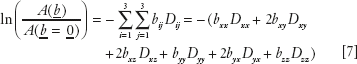
Here, A(b) is the echo magnitude of the diffusion-weighted signal, A(b = 0) is the echo magnitude of the nondiffusion-weighted signal, and bij is a component of the symmetric b-matrix, b. Just as in diffusion imaging, in which a scalar b factor is calculated for each DWI, in DTI a symmetric b matrix is calculated for each DWI. Whereas the b value summarizes the attenuating effect on the MR signal of diffusion and imaging gradients in one direction (40), the b matrix summarizes the attenuating effect of all gradient waveforms (i.e., all imaging and diffusion gradient sequences) applied in all three directions, x, y, and z (47,49,50,51). Just as in diffusion imaging one uses each DWI and its corresponding b factor to estimate an ADC using linear regression of Equation (6), in DTI one uses each DWI and its corresponding b matrix to estimate D using multivariate linear regression1 of Equation (7).
There are two key distinctions one needs to make between diffusion imaging and DTI. In DTI one uses a different experimental design to estimate the diffusion tensor. First, one must apply diffusion gradients along at least six noncollinear and noncoplanar directions (47), whereas in diffusion imaging it is sufficient to apply diffusion gradients along only one direction. Second, one must expand the notion of the b value as well as “cross-terms” that arise between and among imaging and diffusion gradients (49,50). In isotropic media, gradients applied in orthogonal directions do not in principle produce cross-terms, but in anisotropic media they can. This fact had not been considered before.
Finally, it is easy to see that DTI generalizes and subsumes diffusion imaging. If the medium is isotropic, then Dxx = Dyy = Dzz = D and Dxy = Dxz = Dyz = 0. Then Equation (7) reduces to Equation (6) with b = bxx + byy + bzz = Trace(b). More generally, if the medium is not isotropic, then one can show that ADC, D, measured along a direction specified by the unit column vector
 , is given by
 .
.
It is important to note that MRI measurements of the ADC, T1, T2, magnetization transfer rate, proton density, and chemical spectra were all preceded by classical NMR measurements of these quantities, which were first performed decades before their MRI counterpart was introduced. This was not the case with DTI. There were no classical NMR methods developed to measure the self-diffusion tensor or the effective (or apparent) diffusion tensor of water (or other media) in an arbitrary laboratory coordinate system. Thus, the development of DTI (48) first required the invention of a methodology to measure D from the NMR signal (47,52), and then a means to combine this NMR measurement with MRI.
Related posts:
Stay updated, free articles. Join our Telegram channel

Full access? Get Clinical Tree


