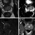
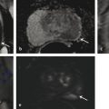
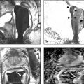
Technical Aspects

Conventional MRI is based on the ¹H signal from water (¹H₂O). Water molecules of the body have constant random brownian motion, a property that is explored by DWI. The high concentration of ¹H₂O provides a strong signal from which an image can be generated. Nonetheless, the contrast mechanism of DWI is distinct from that of conventional MRI. ⁴ DWI studies the displacement of water molecules during the interval between the application of two diffusion-sensitizing gradients. In simple fluids, ¹H₂O diffusion is “free”. However, in biologic tissues, diffusion is restricted given the impedance to the displacement of water molecules, largely by cell membranes. The extent of restriction to motion of water molecules is in proportion to the cellular density ( ▶ Fig. 4.1).

In tissues with less dense cellularity, ¹H₂O can move relatively freely in the extracellular space. ² However, cellularity, and thus the presence of cell membranes, generally increases in tumor tissues. Cell membranes are hydrophobic and act as obstacles to molecular motion of water within the extracellular space, thereby resulting in diffusion restriction.

To measure water motion using DWI, the most common sequence used is a single-shot echo-planar–imaging spin-echo pulse sequence ( ▶ Fig. 4.2), in which rectangular gradient pulses of equal strength are applied before and after the 180-degree refocusing pulse. ⁴ The first gradient pulse causes an initial dephasing of the water molecules. Water molecules that are static will be completely rephased by the second gradient pulse, without any significant change in the measured signal intensity. ² In comparison, water molecules that are moving will not be completely rephased by the second gradient pulse due to the displacement, thus leading to a signal loss on the acquired DWI ( ▶ Fig. 4.2). The strength of these gradient pulses, in part determined by the gradient’s amplitude, is reflected by the b value of the DWI sequence. Use of stronger gradient pulses (indicated by a greater b value) increases the sensitivity of the DWI sequence to water motion.

This paragraph provides sample acquisition parameters for performing DWI. Selection of these parameters must take into consideration the presence of susceptibility and distortion artefacts that are commonly encountered on DW images. ⁴ For instance, the echo time (TE) should be set to the minimum value possible to help reduce such artifacts. Parallel imaging with a reduction factor of 2 (or occasionally 3 if there is a very high signal-to-noise ratio [SNR]) also helps reduce distortion artifacts, in part by allowing for a decreased TE, and thus should routinely be used. The field of view (FOV, approximately 220 × 220 mm) is reduced to fit the prostate. A slice thickness of 3.0 to 3.5 mm and a matrix size of approximately 108 × 108 are used to provide both sufficient SNR and spatial resolution. Oversampling is applied in order to prevent aliasing artifacts that may occur given the reduced FOV. The resulting resolution (approximately 1.2 × 1.2 × 3.5 mm³) allows for the registration of DWI with T2W images, which may help readers identify suspicious foci. ⁵ The receiver bandwidth is set to 1,493 Hz in the readout direction in order to prevent chemical shift artifacts. Multiple slice excitations and signal averages (for instance, 10–20 signal averages) over an extended acquisition duration improve the signal- and contrast-to-noise (CNR) ratios. Using modern systems, it may be possible to obtain different numbers of signal averages for each acquired b value, thereby allowing for obtaining a particularly high number of signal averages for the highest b values in a time-efficient manner. A total acquisition time of 5 to 8 minutes may be reasonable to allow for enough signal averages to attain sufficient SNR.

If a rectal coil is being used, then thinner partitions (2.5 mm) and an even smaller FOV can be acquired, whether at 3T or 1.5T, ⁶ in order to improve spatial resolution and decrease artifacts, despite a resulting loss in SNR and CNR. In evaluating this trade-off, Medved et al showed that the higher spatial resolution (voxel size of 3.1 vs 6.7 mm³) overweighed the decrease in CNR and provided significantly better lesion conspicuity and overall image quality. ⁶ This sequence adjustment may help improve the detection of small or sparse prostate cancers.

Qualitative assessment of prostate DWI consists of a visual assessment of the extent of signal attenuation within tissues on DW images. This assessment incorporates two data sets: the apparent diffusion coefficient (ADC) map and the high b-value source images.

4.3 High b Value Images

Diffusion-weighted images with a high b value (b≥800s/mm²) are routinely acquired in order to increase the conspicuity of tumor foci within the prostate. Higher b values provide greater contrast between tissues based on differences in the extent of signal attenuation of water molecules. At b values less than 800 s/mm², visual detection of tumors using DW images is limited given the strong contributions of T2 weighting to the images at such b values. As a result, the displayed signal intensity reflects both water diffusion and T2 relaxation times. Benign glandular prostate tissue may have a long T2 relaxation time and thus maintains a high signal intensity on DW images that may obscure increased signal intensity within tumors ( ▶ Fig. 4.3). This obscuring of tumors relating to T2 shine-through effects may be commonly encountered even when using a high b value of 800 to 1000 s/mm². One study reported that within this b-value range, tumors were visible in fewer than half of cases. ⁷

One approach to increase tumor visibility is to use a short TE (≤90ms) in order to decrease the T2 weighting and thus reduce the T2 shine-through effect. A more powerful approach to increase the conspicuity of tumor foci is to select an ultrahigh b value (b≥1400 s/mm²), which increases diffusion weighting even further, providing greater suppression of the benign prostate ( ▶ Fig. 4.4) and thus improving the sensitivity of source DW images for PCa detection compared with standard high b values ( ▶ Fig. 4.5).

In a study of 41 patients with biopsy-proven prostate cancer imaged at 3T with 5 b values (0, 1000, 1500, 2000, 2500 s/mm²), Metens et al reported the highest tumor visibility at b = 1500 s/mm² and b = 2000 s/mm², as well as the best CNR at b = 1500 s/mm², thus supporting the use of ultrahigh b values. ⁸ Likewise, in a study of 201 patients undergoing radical prostatectomy as the reference standard, Katahira et al showed a significantly higher sensitivity (73.2%), specificity (89.7%), and accuracy (84.2%) using b = 2000-s/mm² images than using b = 1000-s/mm² images (sensitivity: 61.2%, specificity: 82.6%, accuracy: 75.5%), for results pooled among three independent readers. ⁹ Such results were confirmed in the study by Rosenkrantz et al, who showed, in a series of 29 patients, also with radical prostatectomy serving as the reference standard, the significantly higher sensitivity of DW images, interpreted by two independent readers, acquired at b = 2000 s/mm² compared to those acquired at b = 1000 s/mm² for detecting tumor foci. ¹⁰

Despite the value of ultrahigh b values for tumor detection, the direct acquisition of such b values is challenging. As the b value passes 1000 s/mm², the presence of artifacts increases to potentially very pronounced levels, and the SNR may become very low, thereby degrading image quality. A longer TE may be required in order to acquire ultrahigh b-value DW images on some systems, thereby contributing to the greater distortions artifacts. While more signal averages may be used to help maintain sufficient SNR, this in turn prolongs the overall scan time. Sufficient SNR at ultrahigh b values is optimally provided through use of a 3-T system or use of an endorectal coil at 1.5T. To circumvent this limitation, an alternative solution is to calculate the ultrahigh b-value (≥ 1400 s/mm²) images from a set of lower b-value images by extrapolating the signal decay of the DW curve. This approach is already commercially available on some MR platforms ( ▶ Fig. 4.6). These computed ultrahigh b-value DW images provide the image contrast of directly acquired ultrahigh b-value images, which helps improve tumor detection, yet without any additional acquisition time in comparison with that needed to acquire standard b-value images. Furthermore, these images avoid the technical challenges inherent in avoiding greater distortion artifacts when directly acquiring the ultrahigh b-value images, for instance, not requiring any adjustment in TE.

Several studies report clinical utility of computed ultrahigh b values, using as a reference standard either biopsy findings ^{11​ 12} or histology from radical prostatectomy. ¹³ For instance, Maas et al in a series of 42 patients with biopsy-proven PCa, imaged at 3T using a pelvic phased-array coil, reported that the CNR of acquired and computed DWI at a b value of 1400 s/mm² was similar. ¹¹ They concluded that calculated DWI could be used in place of acquired DWI at b = 1400 s/mm² as a means of increasing the conspicuity of tumor foci. Moreover, the authors also showed that lesion conspicuity could be improved even further using calculated DW images by increasing the calculated b value up to 5000 s/mm² ( ▶ Fig. 4.7).

These results were confirmed in the study by Rosenkrantz et al performed at 3T using a pelvic phased-array coil and acquired b values of 50, 1000, and 1500 s/mm². ¹³ The authors reported that the numerous measures of quality and diagnostic performance of the DW sequence (suppression of benign tissue, reduced distortion, absence of artifacts, sensitivity, and positive predictive values for tumor detection and tumor-to-peripheral zone contrast) were equal or superior using computed DW images at b = 1500 s/mm² than using the directly acquired b = 1000- or 15000-s/mm² images for interpretation by two independent readers.

In a third study of 106 patients with PCa proven by MRI-TRUS image fusion biopsy, Grant et al compared acquired and calculated b = 2000 s/mm² images at 3T. ¹² Although image quality was slightly inferior for the calculated images in their study, tumor visibility was similar between the two image sets.

Given these considerations, it currently is recommended to incorporate some implementation of ultrahigh b-value DWI (b≥1400 s/mm²) within routine clinical protocols. Depending upon the gradient performance, coil design, and software platform, DWI with directly acquired b values greater than 1000 s/mm² may be prohibitive in clinical practice. Thus, the feasibility of incorporating ultrahigh b-value DWI is facilitated by computed DWI. However, computed DWI is not currently available for all MR systems. Thus, some practices will still need to acquire these ultrahigh b-value DWI directly, taking all steps possible to reduce associated artifacts. One important measure that helps to decrease distortion artifacts on DWI is ensuring that the rectum is empty of air. If an endorectal coil is used, then it is recommended to inflate the coil with perfluorocarbon or fluids containing manganese, such as pineapple juice, which substantially lessen the signal brightness on T2W and DW sequences. When not using an endorectal coil, technologists should be trained to instruct the patient to evacuate their rectum before starting the examination. Additional approaches that some practices employ to help reduce rectal gas for non–endorectal coil exams include administration of a rectal laxative 1 to 2 hours before the MRI, and aspiration of rectal gas using a female bladder catheter just before the examination, once the patient is on the table. Although not standard among all centers, such simple precautions may help ensure a collapsed rectum in most cases.

It is anticipated that continued improvements in MRI hardware and software will improve the quality of acquired DWI and the clinical availability of computed DWI, which in turn will enhance the diagnostic performance of mpMRI. For instance, DWI at b ≥ 1400 s/mm² may help differentiate prostate cancer from focal prostatitis in the peripheral zone (PZ) ( ▶ Fig. 4.8) and possibly from stromal benign prostatic hyperplasia (BPH) nodules in the transition zone (TZ) ( ▶ Fig. 4.9).

Whereas prostatitis and stromal BPH often show increased signal on DWI at b = 1000 s/mm², this signal (for prostatitis more so than for stromal BPH) is more likely to be suppressed at ultrahigh b values. In comparison, prostate cancer, given its increased degree of impeded diffusion relative to these benign entities, remains hyperintense at the ultrahigh b values. Thus, it is expected that incorporation of DWI at b ≥1400 s/mm² may improve the diagnostic performance of the Prostate Imaging–Reporting and Data System (PI-RADS) particularly in the characterization of equivocal lesions (PI-RADS assessment category 3).

4.4 The Apparent Diffusion Coefficient Map

Data obtained from DWI performed at different b values allows for a quantitative analysis. Although such an analysis is possible using only two b values, three b values are most commonly obtained in clinical practice: one low (50 or 100 s/mm²), one intermediate (400 or 500 s/mm²), and one high (800 or 1000 s/mm²). A b value of 0 is generally avoided for the low b value in order to avoid the influence of the early capillary component on the measured diffusion signal (see below). By plotting the logarithm of the measured signal intensity on the y-axis against the b values on the x-axis, a line can be traced through the points for each of the acquired b values whose slope characterizes the ADC of the given tissue ( ▶ Fig. 4.10).

The ADC is interpreted to represent the net displacement of water molecules over a timescale reflecting the diffusion-sensitizing gradients applied during the DWI acquisition. The use of several b values helps improve the fit of the curve and potentially minimize errors in the ADC calculation. Current MR systems and workstations can automatically calculate the ADC value for each pixel and display the results as a parametric map. The ADC map is not affected by the T2 shine-through effects that impact the source DW images. However, measured ADC values are inversely correlated with the highest b-value used during the acquired sequence. Regions of interest are used to obtain ADC measurements within suspicious focal areas within the prostate. Low ADC values within an area indicate the presence of restricted diffusion. Such areas exhibit a low signal intensity on the ADC map in contrast with their high signal intensity on the source DW images, in both instances reflecting the same underlying phenomenon ( ▶ Fig. 4.8; ▶ Fig. 4.11).

Several studies have evaluated the b value that optimizes tumor visibility on the ADC map. Kim et al. ¹⁴ reported in a series of 48 patients that focal lesions were more conspicuous on the ADC map when constructed from a maximal b value of 1,000 s/mm² than from one of 2,000 s/mm². Similarly, Kitajima et al ¹⁵ reported that in 26 patients with biopsy-proven PCa, the lesion conspicuity on the ADC map calculated using a maximal b value of 2000 s/mm² was not superior to that calculated using a maximum b value of 1000 s/mm². Moreover, Rosenkrantz et al ¹⁰ despite observing a higher diagnostic performance of source b = 2000 s/mm² images than of source b = 1000 s/mm² images, reported no difference in sensitivity from a visual analysis between ADC maps calculated using these two b values (p≥0.309).

These findings suggest that calculation of the ADC map should not incorporate b values > 1, 000 s/mm². Even if using b values up to 1000 s/mm², the optimal selection of b values within this range remains controversial. Thormer et al ¹⁶ evaluated 41 patients with biopsy-proven PCa at 3T using an endorectal coil before prostatectomy. Four combinations of b values (0–800, 50–800, 400–800 and 0–50–400–800 s/mm²) were used to calculate the ADC map, and tumor conspicuity was visually assessed on each map by three independent radiologists. The best tumor conspicuity was obtained with ADC maps calculated from b values of 50–800 s/mm², followed by b values of 0–800 s/mm². Currently, the PI-RADS version 2 guidelines recommend acquiring three b values (low, intermediate, and high, as previously noted), avoiding a b value of 0. While incorporation of an ultrahigh b value is also advised, this should not be acquired as part of the multi–b-value DWI acquisition that is used for generating the ADC map. Rather, if the ultrahigh b-value images cannot be computed from the acquired lower b-valuedata, then it is advised that direct acquisition of the ultrahigh b-value images be accomplished in a second, separate DW acquisition comprising solely the ultrahigh b-valuedata, thus excludeing this data from the ADC map calculation.

4.5 Quantitative Assessment of Prostate Diffusion-Weighted-MRI in the Peripheral Zone

Numerous studies have investigated the potential added value of quantitative ADC metrics to not only improve the diagnostic accuracy of tumor detection and localization compared with a visual assessment but also to determine tumor aggressiveness.

4.5.1 Diagnosis of Prostate Cancer

An initial publication reported that the mean ADC value was significantly lower in PCa than in benign tissue. ¹⁷ Subsequently, many articles have confirmed the presence of a significant difference. ^{17,​ 18,​ 19,​ 20,​ 21,​ 22,​ 23,​ 24,​ 25,​ 26} However, the reported values of ADC in prostate cancer show great variation, ranging from 0.98± 0.22 x 10^–3mm²/s to 1.39 ± 0.23 x 10^–3mm²/s. ^{24,​ 25} One factor contributing to this variation is the selection of b value among the studies, given that ADC values are lower when computed using higher maximimum b values. For instance, in the study by Vargas et al, ²⁷ ADC values were lower at b = 1000 s/mm² than at b = 700 s/mm², and in the study by Kitajima et al, ²⁸ ADC values were lower at b = 2000 s/mm² than at b = 1000 s/mm². Thus, it could be anticipated that two ^{20,​ 21} of the three studies performed using a maximum b value up to 600 s/mm^{2 19,​ 20,​ 21} show higher ADC values, (1.33 ± 0.32 and 1.43 ± 0.19 × 10^–3mm²/s) in cancer than those studies performed using a maximal b value > 600 s/mm². However, even above 600 s/mm², the ADC values continue to exhibit much variation among protocols using comparable acquisition parameters. The studies by Kumar et al ²⁴ and Desouza et al, ²² which used only slightly different protocols (five and four b values, high b values of 1000 and 800 s/mm², respectively), provide a representative example, as the mean ADC values in cancer were substantially lower in the study by Kumar et al than in that of Desouza et al (0.98 ± 0.22 x 10^–3mm²/s vs. 1.30 ± 0.30 x 10^–3mm²/s) and the obtained cutoff values for differentiating cancer from benign tissue were substantially different (1.17 x 10^–3mm²/s vs. 1.36 x 10^–3mm²/s, respectively). Another finding shared by essentially all of these studies is that despite the significant difference of ADC values between cancer and benign tissue, an overlap in ADC values exists between benign and malignant tissue in individual patients, with this overlap potentially being substantial. This concern was particularly well illustrated in a study by Nagel et al ²⁹ that evaluated 88 consecutive patients having suspicious focal areas on mpMRI (3T, pelvic phased-array coil, b values of 0, 100, 500, and 800 s/mm²) and in whom 116 biopsy cores were obtained by MR-guided biopsies. The mean ADC value of normal tissue (1.22 ± 0.21 × 10^–3mm²/s) was higher than that of both benign prostatitis (1.08 ± 0.18 x 10^–3mm²/s, p<0.001) and of PCa (0.88 ± 0.15 x 10^–3mm²/s, p<0.001). However, considerable overlap was observed between prostate cancer and prostatitis. No difference in ADC value was demonstrated between low-grade cancer (Gleason score <7) and high-grade cancer (any percentage of Gleason pattern 4), which may explain, at least in part, the suboptimal performance of ADC values in identifying prostate cancer.

Given the published studies, reliably differentiating cancer from benign foci purely on the basis of measurements of the absolute ADC value seems difficult if not impossible at present. Thus, detection of prostate cancer continues to largely rely on a visual assessment of both the signal intensity on ultrahigh b-value DW images combined with a visual assessment of the ADC map, as is recommended by PI-RADS version 2.

4.5.2 Apparent Diffusion Coefficient Map and Peripheral Zone Tumor Aggressiveness

Partly related to the very large increase in the number of men undergoing sextant prostate biopsies over the recent decades, many men are currently being diagnosed with indolent or nonsignificant prostate cancer that will not impact survival or cause harm. ³⁰ These tumors do not require radical treatments, which are associated with potential side effects including incontinence and impotence that greatly impact patients’ quality of life. Diffusion-weighted magnetic resonance imaging, in addition to clinical, biochemical, and pathologic features, may aid in establishing the aggressiveness of prostate cancer and help predict those tumors most likely to progress rapidly. While tumor grade is the primary determinant of tumor aggressiveness (in particular, presence of a component with a Gleason score of 4 or 5), tumor volume and extraprostatic extension are also important considerations.

4.5.3 Apparent Diffusion Coefficient Map and Gleason Score of Peripheral Zone Tumors

Many studies have investigated the ability of ADC values to predict tumor Gleason score using biopsy results as the reference standard. ^{20,​ 21,​ 23,​ 31,​ 32,​ 33,​ 34,​ 35,​ 36,​ 37} However, such studies are suboptimal given that sextant biopsies can miss high Gleason grades in approximately 30% of cases. Magnetic resonance–targeted biopsies (in-bore or using MRI-TRUS image registration ³⁴) may provide a more appropriate reference standard but, are also limited: small amounts of Gleason pattern 4 (up to 20%) can be missed, ³⁸ and in the author’s experience, ³⁹ Gleason score 3+4 tumors on fusion biopsy having a Gleason pattern 4 30% are commonly upgraded to Gleason score 4+3 at pathologic examination of prostatectomy specimens.

As a result, the most robust way of evaluating the ability of ADC values to estimate the Gleason score as well as the percentage of Gleason pattern 4 is to correlate ADC metrics with findings from the pathologic examination of the radical prostatectomy specimen. Indeed, such an association has been performed in nearly 20 studies as of this writing. ^{27,​ 40,​ 41,​ 42,​ 43,​ 44,​ 45,​ 46,​ 47,​ 48,​ 49,​ 50,​ 51,​ 52,​ 53,​ 54,​ 55} While the maximimum b value used for DWI acquisition was 800 to 1,000 s/mm² in the majority of these studies, important variation in selection of intermediate b values is apparent. Indeed, many of the studies used only two b values (commonly 0 and 1000 s/mm²). The use of only two b-values is likely to be, at least partly, vendor dependent given the lack of multi–b-value functionality of DWI on many MR platforms at the time of the publication of the articles.

All of the studies agree that there is an inverse relationship between the ADC value and the Gleason score, with a correlation coefficient that varies from 0.32 (weak correlation) to 0.50 (fair correlation). In studies that specifically compare ADC values of Gleason score 6 tumors to those of Gleason score > 7 tumors, ^{27,​ 40,​ 43,​ 44,​ 45,​ 51,​ 53,​ 55} the ADC value of Gleason score 6 tumors is significantly higher, measuring above 1.0 x 10^–3mm²/s in all studies but one, ⁴⁰ with values ranging from 1.0 to 1.3 x 10^–3mm²/s, compared with that of Gleason score > 7 tumors (ADC values ranging from 0.69 to 0.88 x 10^–3mm²/s).

Some of these studies aimed to achieve even greater precision, exploring the ability of ADC values to characterize intermediate-grade tumors (Gleason score 7), which has consistently presented a greater challenge for DWI than separating low- and high-grade tumors. For this purpose, limitations of TRUS-guided biopsies are well known: Gleason score 6 tumors can be upgraded to Gleason score 7 at surgical pathology in at least 25% of cases, and Gleason score 3+4 tumors can be upgraded to Gleason score 4+3 tumors in 20 to 66% of the cases. ⁵⁶ Being able to detect the most aggressive foci within an individual tumor using DWI conceptually should improve the accuracy in differentiating Gleason score 3+4 and Gleason score 4+3 tumors, which is clinically important given the well-established poorer prognosis of tumors with Gleason score 4+3 compared to those with Gleason score 3+4. ^{57,​ 58,​ 59} Furthermore, the percentage of Gleason pattern 4 (%G4) may also provide a useful marker of tumor aggressiveness as reported by Stamey et al, ⁶⁰ who demonstrated that biological progression after radical treatment increased for each 10% increment of %G4. Cheng et al similarly showed that the percentage of Gleason pattern 4 and 5 could predict survival after radical prostatectomy. ⁶¹

The accuracy of ADC values in discriminating Gleason scores of intermediate-grade tumors from those of lower- or higher-grade tumors varies across studies. Yoshimitsu et al ⁵⁵ failed to find a significant difference in ADC values between tumors with Gleason scores 6 and 7 or between tumors with Gleason scores 7 and 8. While a number of studies ^{27,​ 43,​ 45,​ 48,​ 50,​ 53} have compared ADC values between tumors with Gleason scores of 3+4 and 4+3, results of these studies have been discrepant. Verma et al ⁵³ and Rosenkrantz et al ⁵⁰ failed to show a significant difference between the two groups, while four studies ^{27,​ 43,​ 45,​ 48} found a significant difference. These discrepancies probably relate, at least in part, not only to differences in the MRI protocol across studies but also to varying amounts of Gleason pattern 4 among included patients having a Gleason score of 3+4. Intuitively, it may indeed be expected that tumors with small amounts of Gleason pattern 4 (up to 20 to 25%) may have a mean ADC value similar to that of Gleason 6 tumors given potential sparse distribution of the Gleason pattern 4 component, thereby making it virtually impossible to detect by imaging an area within the tumor having more restricted diffusion as a marker of the Gleason pattern 4 component. Moreover, even in studies that did report the ability to differentiate intermediate- from lower- and higher-grade tumors using ADC values, substantial overlap between the subclasses was noted, as supported by reported high standard deviations of ADC values within the groups.

In order to circumvent these limitations, Rosenkrantz et al recently proposed a potentially improved approach to evaluating the ADC map ⁵⁰ in a study of 70 patients imaged before prostatectomy at 3T using a pelvic phased-array coil. Instead of measuring the mean ADC value on a single slice, the authors measured the whole-tumor ADC using in–house-developed software that allows placement of three-dimensional volumes of interest (VOIs) incorporating tumor voxels across multiple slices. From these measurements, the number of voxels having a given ADC value can be normalized to the total number of voxels within the VOI, allowing for computation of the so-called ADC entropy, which reflects the textural heterogeneity of the tissue. In that study, ADC entropy was significantly higher in Gleason score 4+3 tumors than in Gleason score 3+4 tumors, although mean ADC was not significantly different between the groups.

4.5.4 Apparent Diffusion Coefficient Ratio and Gleason Score

The ADC ratio refers to the ratio of the mean ADC value of the tumor itself to the ADC value of a surrounding reference tissue. Computation of the ADC ratio is intended to provide intrapatient normalization of ADC measurements and potentially compensate for equipment-related variations and thereby improve discriminatory performance compared with absolute ADC values. One approach to obtaining the ADC ratio entails placement of region of interest in the contralateral benign PZ, in mirror position to the tumor.

As with absolute ADC metrics, there is conflicting data regarding the value of ADC ratios. Lebovici et al, in a series of 22 men imaged at 1.5T using an endorectal coil and transperineal 20-core saturation biopsy protocol serving as the reference standard, showed that the ADC ratio performed better than the ADC value in the PZ to discriminate Gleason score 8–9 from Gleason score 6–7 tumors. ⁶² In that study, the mean ADC ratio for high-grade tumors was significantly lower (0.40 ± 0.09) than that of low- and intermediate-grade tumors (0.54 ± 0.09). Furthermore, the area under the curve (AUC) for differentiating these two tumor groups was 0.90 for the ADC ratio, compared with 0.75 for the ADC value. Similarly, Thormer et al, ⁵² in a series of 45 patients imaged at 3T using an endorectal coil (b values: 50–500–800 s/mm²) prior to prostatectomy reported that a cutoff value of the ADC ratio of 0.46 allowed for a correct characterization of 79% of tumors, performing better than TRUS-guided sextant biopsies, which only correctly characterized 75% of tumors. In addition, the AUC of the ADC ratio (0.90) was superior to that of the ADC value (0.79). However, these results were not confirmed by De Cobelli et al, ⁶³ who correlated the ADC value and the ADC ratio (b values: 0–800–1600 s/mm²) with the surgical Gleason score at 1.5T using an endorectal coil in 39 patients. The AUC was 0.92 (p = 0.12) for the ADC value and 0.86 for the ADC ratio (p = 0.42), indicating no incremental value of the ADC ratio compared to that of the ADC value. Finally, in a study by Rosenkrantz et al of 58 patients imaged before radical prostatectomy in which two independent observers performed ADC value and ADC ratio assessments separately in the peripheral zone and transition zone, ADC values significantly outperformed ADC ratios in the PZ for both readers, whereas the two approaches had mixed results among the two readers in the TZ. ⁶⁴

In assessing the relevance of ADC metrics for differentiating prostate cancer from benign PZ tissue and for evaluating tumor aggressiveness, Scheenen et al ⁶⁵ emphasized that two distinct parameters ( ▶ Fig. 4.2) impact the strength of the diffusion-sensitizing gradients applied during a DW sequence: the diffusion time, which is the time interval between the two pulsed field gradient lobes, and the gradient duration, which is the overall time interval during which the gradients are applied. The ADC value is derived from the decay of the MR signal during this interval and thus can be influenced by either of these two parameters. Following a qualitative visual evaluation of the ADC map, further incorporation of quantitative ADC measurements for tumor characterization must therefore be done with caution. The ADC value not only depends linearly on the diffusion time, but also on the square of the gradient duration. Therefore, quantitative measurements of the ADC of prostate cancer and of benign tissue optimally should be compared between patients for which both the diffusion time and gradient duration were the same. However, in routine practice, it is difficult to determine when this condition is indeed the case, as these parameters are integrated together via the b value, reflecting a composite of the two parameters, and their separate values are typically not accessible to the radiologist.

Despite these limitations, we suggest that use of two particular threshold values in terms of ADC measurements may remain clinically helpful when employing a standardized DWI protocol, as recommended in PI-RADS version 2 computation of the ADC map from a low (not b = 0), intermediate, and high (b = 800 – 1000 s/mm², but not higher) b value. First, above an ADC measurement of approximately 1.1 to 1.2 x10^–3 mm², significant tumor is uncommon ( ▶ Fig. 4.12). ⁶⁶ Second, below an ADC measurement of approximately 0.850 x10^–3 mm²/s, high-grade cancer with more than 20 to 25% G4 can be suspected ( ▶ Fig. 4.13). ⁴⁶ These two threshold values may help guide decisions regarding whether to perform biopsy of PI-RADS category 3 lesions as well as may indicate the presence of a high Gleason pattern component that may or may not be not identified on the biopsy findings.

Related posts:

Introduction to Prostate Cancer: Clinical Considerations PET/CT and PET/MR Imaging Evaluation of Prostate Cancer Prostate Cancer Pathology Prebiopsy MRI and MRI-Targeted Biopsy Dynamic Contrast-Enhanced MRI of the Prostate Introduction to Prostate MRI Protocols: Hardware, T2-Weighted Imaging and MR Spectroscopy

Stay updated, free articles. Join our Telegram channel

Join