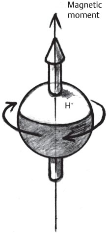
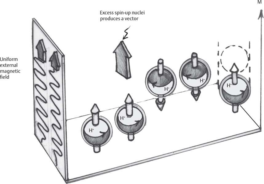
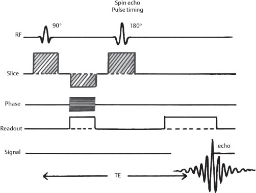
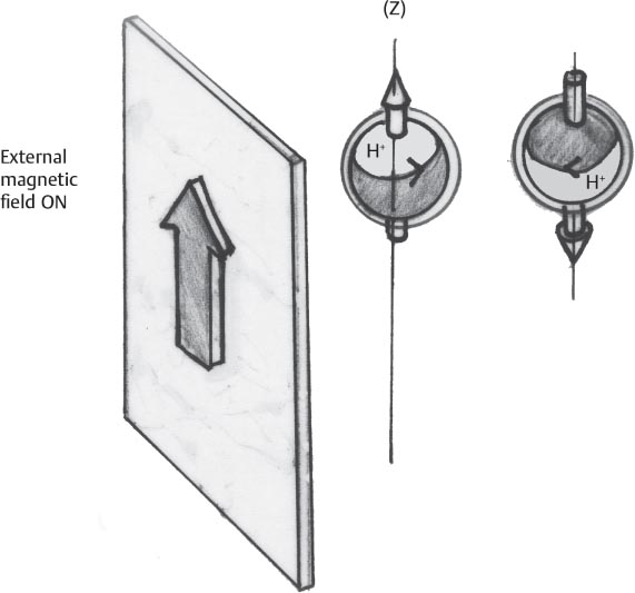
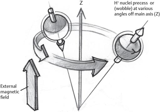
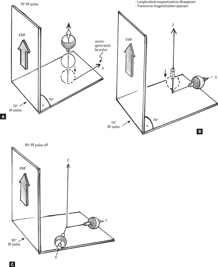
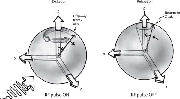
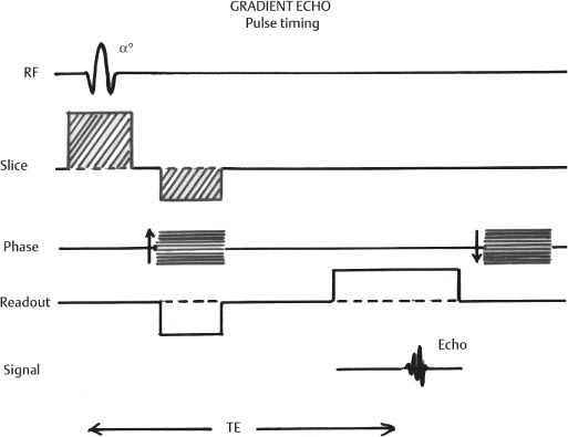
Essentials of MRI Physics and Pulse Sequences

1 Essentials of MRI Physics and Pulse Sequences

Rick W. Obray, Douglas P. Beall, John D. Reeder, John A. Carrino, and Laura M. Fayad

MRI is an essential tool in the accurate diagnosis and treatment of musculoskeletal disease. The number of MRI applications has increased dramatically over the past two decades and will likely continue to increase. A detailed understanding of the fundamentals of MRI physics is not required to review images, although a basic working knowledge of certain key principles is important for the accurate utilization of the technology. This chapter provides the reader with a basic understanding of the physics behind MRI by addressing specific applications of MRI within musculoskeletal radiology and emphasizing how an MR image is generated and what basic sequences are important for optimally showing musculoskeletal anatomy. The intent is to provide the reader with a sufficient working knowledge of the technology to allow for the acquisition of high-quality images in a reasonable amount of time. This chapter is only a brief introduction to what most would consider a complex technology, and the reader is referred to additional sources for more detailed explanations.1–6

Fundamentals of MRI

Magnetization of Nuclei and Tissues and the Larmor Equation

Understanding how an MR image is generated requires some knowledge of the basic physical properties of the nucleus of an atom and its components, that is, neutrons and protons. All neutrons and protons within the nucleus spin about their axes and generate a magnetic field called a magnetic dipole (Fig. 1.1). The magnetic dipoles of protons and neutrons of even-numbered nuclei cancel each other out. However, odd-numbered nuclei generate a magnetic moment, which can be represented as a vector. When placed in a magnetic field, odd-numbered nuclei, because of their magnetic moments, align parallel to the external magnetic field in one of two orientations: spin-up or spin-down (Fig. 1.2). A small excess of nuclei align in a spin-up orientation (slightly greater stability) and generate an overall small net magnetization vector (Fig. 1.3). Conveniently, the human body is replete with hydrogen, a ubiquitous atom with odd-numbered nuclei (hydrogen has one proton and no neutrons) and, to a lesser extent, with fluorine. It is the manipulation within an external magnetic field of this small number of excess spin-up, odd-numbered nuclei that is the basis for the signal that ultimately generates an MR image.^1,2

When spinning nuclei are exposed to an external magnetic field, the magnetic fields of the spinning nuclei and the external magnetic field interact and cause the nuclei to precess, or “wobble” (Fig. 1.4). The frequency of precession can be described by the Larmor equation:

where ω₀ is the precessional frequency, B₀ is the external magnetic field strength measured in tesla (T) units, and γ is the gyromagnetic ratio measured in megahertz per tesla unit. Conveniently, the ω₀ is constant for every atom at a particular magnetic field strength, and it is key for the localization of the MRI signal within space (see details below).

When an RF pulse (at the Larmor frequency for hydrogen at a given field strength) is applied within an external magnetic field, the net magnetization vector flips from its longitudinal direction by a certain angle (flip angle). This flipping process produces a transverse magnetization vector (perpendicular to the external magnetic field) and a longitudinal magnetization vector (parallel to the external magnetic field) (Fig. 1.5). The magnitude of the flip angle is determined by the strength and duration of the RF pulse applied. A 90-degree RF pulse, for instance, aligns the magnetization vector in a plane perpendicular to the external magnetic field, whereas a 180-degree RF pulse aligns the magnetization vector in a plane parallel to but in a direction opposite to that of the external magnetic field. After the RF pulse, the precessing nuclei initially are also “in phase” with one another; that is, they are precessing in synch with one another. This synchronized precession maximizes the transverse magnetization vector (additive effect). Once the RF pulse is turned off, the precessing nuclei relax, the longitudinal vector returns, and the transverse vector dissipates (Fig. 1.6). The transverse magnetization vector produces a signal as it precesses around a receiver coil; this signal can be optimized, recorded, and ultimately transformed into MRI images by Fourier analysis.¹

Fig. 1.1 Neutrons and protons within the nucleus spin about their axes and generate a directional magnetic field called a magnetic dipole. In this illustration, the dipole is pointing upward.

Fig. 1.2 Odd-numbered nuclei may exist in one of two energy states when placed in an external magnetic field: spin-up or spin-down orientation, that is, parallel to and aligned with the external magnetic field (large arrow) or parallel to and in an opposite direction to the external magnetic field. The spin-up orientation (z), is a slightly more stable energy state.

Fig. 1.3 The slight excess nuclei in the spin-up orientation is the result of the increased stability of the spin-up orientation relative to the spin-down orientation, and it produces a net magnetization vector (large arrow) that can be manipulated to create an RF signal, which in turn can be used to create an MR image. The two smaller arrows depict the direction of the external magnetic field (M).

Fig. 1.4 All nuclei, including hydrogen nuclei, precess about their axes when placed in an external magnetic field, which is similar to a “spinning top.” The frequency of precession is related to the strength of the external magnetic field as determined by the Larmor equation (ω₀= B₀ × γ).

In summary, by using an RF pulse to flip the excess spin-up hydrogen nuclei and ultimately transform the longitudinal magnetization vector within a sample or tissue into a transverse magnetization vector, an RF signal can be generated and subsequently used to create an image.

T1, T2, and T2*

The transverse and longitudinal magnetization vectors and the generation of the MRI signal should be addressed in terms of how they relate to T1, T2, and T2*. When an RF pulse that is interacting with nuclei in an external magnetic field is turned off, the precessing nuclei return to their original equilibrium state and realign with the external magnetic field. As one might expect, the longitudinal magnetization vector returns to equilibrium value before the RF pulse does. The return or recovery of the longitudinal magnetization is known as T1 recovery, with T1 being defined as the time constant representing 63% recovery of the equilibrium longitudinal magnetization vector.2 Conversely, after the RF pulse is turned off, the transverse magnetization vector decays exponentially, with a decay rate constant, or T2. The T2 decay relates to spin dephasing secondary to the interaction of the local magnetic fields of the individual nuclei. The time necessary for T2 decay quantitatively represents the time in which the transverse magnetization vector has decayed by 63% of its maximum. The T1 relaxation time is also known as the longitudinal or spin-lattice relaxation, and T2 is also known as the transverse or spin-spin relaxation. The T2* relaxation time represents the loss of the transverse magnetization vector secondary to T2 effects and the spin de-phasing secondary to local magnetic field inhomogeneities. Therefore, the T2* relaxation time is always shorter than T2. As would be expected, T1, T2, and T2* differ for individual tissues. Tissues with a long T1 include water and large protein molecules, and tissues with a short T1 include fats and intermediate-size molecules. Tissues with a long T2 include liquids, whereas large molecules and solids generally have short T2 times. The T2* relaxation time usually is short for fat and water.^2,3

In summary, individual tissues, such as fat and water, have reasonably well-defined T1, T2, and T2* time constants related to the recovery of the longitudinal magnetization signal (T1) and the decay of the transverse magnetization signal (T2, T2*) after an RF pulse. These differences in T1, T2, and T2* directly impact the strength of the RF signal emitted from a particular type of tissue (e.g., fat or water) at a given time and ultimately can be converted to visual differences in tissue contrast on the final image.^2,3 It is MRI’s ability to resolve subtle differences in the T1, T2, and T2* characteristics of various tissues and assign the differences to a discrete location (pixel/voxel, see below) within the patient that allows MRI to produce images of such high spatial resolution and to provide information about the anatomy and pathology within the musculoskeletal system.

Gradient Coils and Signal Localization

The transverse magnetization signal is localized within tissue via the use of gradient coils. Nuclei in an external magnetic field precess at a particular frequency when subjected to an RF pulse, as described by the Larmor equation. By altering the external magnetic field and creating gradients in the x, y, and z planes, it is possible to identify the location of signal within tissue based on its emitted RF and phase. Gradient coils superimpose small field gradients in the x, y, and z directions on the main magnetic field and include section-selection gradients, phase-encoding gradients, and frequency-encoding gradients.¹ Section-selective gradients select the section to be imaged.¹ The phase-encoding gradient causes a phase shift that allows for localization of the signal by its phase. A frequency-encoding gradient causes a frequency shift, allowing for localization by frequency.¹ The determination of which plane (i.e., x, y, z) each gradient is applied depends on the orientation of the image (i.e., axial, sagittal, coronal).^1,4 Data within the MR image are divided into pixels and voxels, which localize the signal in two or three dimensions, respectively. A pixel is a 2D unit in the x-y, x-z, or y-z planes, whereas a voxel is a 3D unit, representing a unit of volume within the data set/image.

Fig. 1.5 Manipulation of the magnetization vector (EMF, external magnetic field). (A) An external RF pulse administered at the Larmor frequency can flip the direction of the magnetization vector from the longitudinal to the transverse direction. (B) The longitudinal component of the magnetization vector decreases and the transverse component of the magnetization vector increases, based on the strength and duration of the applied RF pulse. The angle the net magnetization vector makes with the longitudinal axis, that is, the external magnetic field, is called the flip angle. (C) A 90-degree RF pulse, for instance, will flip the direction of the net magnetization vector 90 degrees relative to the external magnetic field.

Fig. 1.6 After the discontinuation of an RF pulse, the net magnetization vector will relax, or return, to a more stable energy state, with recovery of the longitudinal component and loss of the transverse component of the magnetization vector. The strength of the transverse component of the magnetization vector is what is ultimately used to generate the MR image.

MRI Pulse Sequence and TE, TR, and Inversion Time

An MRI pulse sequence is the sequence of RF pulses and magnetic field gradients used to generate an image, and several concepts in addition to those discussed above are important when interpreting an MRI pulse sequence: TE, TR, and inversion time.

In conventional SE and gradient-echo sequences, the TE is the time from the initial RF pulse (used to flip the longitudinal magnetization vector into the transverse plane/transverse magnetization vector) to the center of the echo signal (time when signal is at its maximum) (Fig. 1.7). In conventional SE sequences, a phase-encoding gradient is applied at TE/2 to allow for spin rephasing at TE. This technique maximizes the recorded signal at readout (Fig. 1.7). In gradient-echo sequences, gradients are used to “recall the echo” at TE and use a negative gradient followed by a positive gradient (gradient echo) to refocus the signal at readout (Fig. 1.8). One might question why it is necessary to refocus at all. The transverse magnetization degrades secondary to dephasing effects, as described above, and is represented quantitatively by T2 and T2*. Dephasing weakens the transverse magnetization vector/signal, and rephasing (using a perfectly timed gradient echo) rephases, or resynchronizes, the precessing nuclei. When all the nuclei are in phase, or precessing in synch (i.e., vectors pointing in the same direction), the recorded signal is at a maximum. TE primarily affects T2 in conventional SE sequences and T2* in gradient-echo sequences.^1,2

Fig. 1.7 In this example of a conventional SE pulse sequence, the top line shows an RF pulse sequence, a 90-degree pulse followed by a 180-degree refocusing pulse. Section-selection gradients, a phase-encoding gradient, and a readout or frequency-encoding gradients are also shown. The bottom line depicts the RF signal or “echo” recorded at TE. The 180-degree pulse is responsible for the echo at a specific time, that is, TE.

Fig. 1.8 In this example of a standard gradient-echo pulse sequence, the top line shows the RF pulse resulting in a predetermined flip angle. Section-selection gradients, a phase-encoding gradient, and readout or frequency-encoding gradients also are shown. A refocusing gradient (readout or frequency selection gradient sequence), which refocuses signal, produces an echo at TE, hence the name gradient echo.

TR is the time interval between the initial RF pulse of the basic pulse sequence and the subsequent repetition of the initial RF pulse.1 In conventional SE sequences, TR primarily affects T1 or the recovery of the longitudinal magnetization vector.

Only gold members can continue reading. Log In or Register to continue