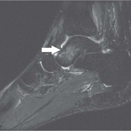
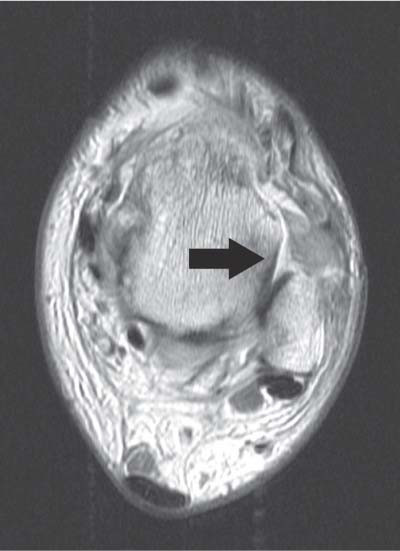
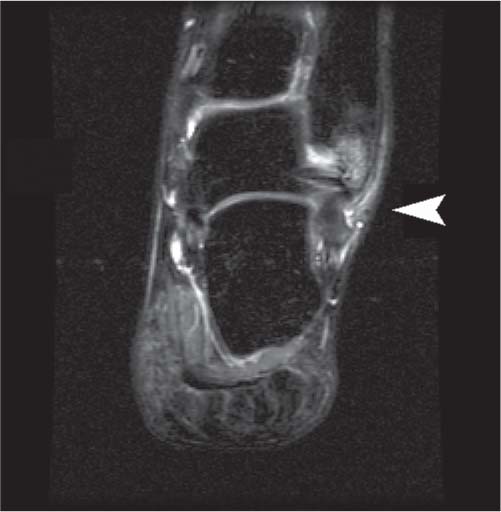
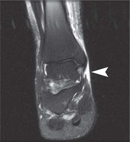
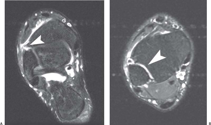
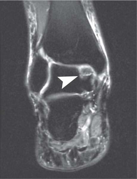
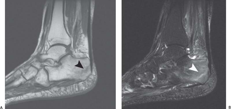
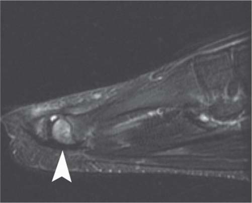
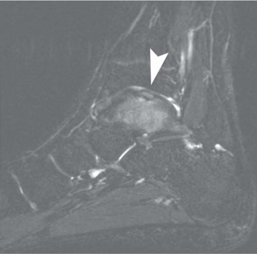
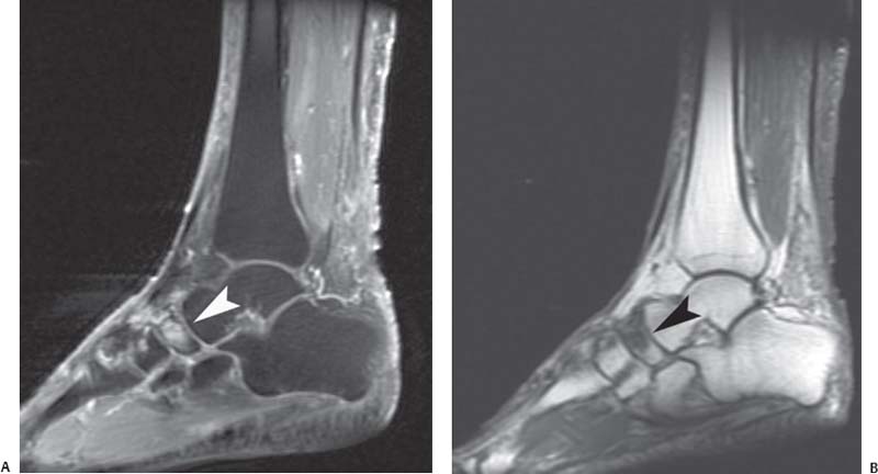
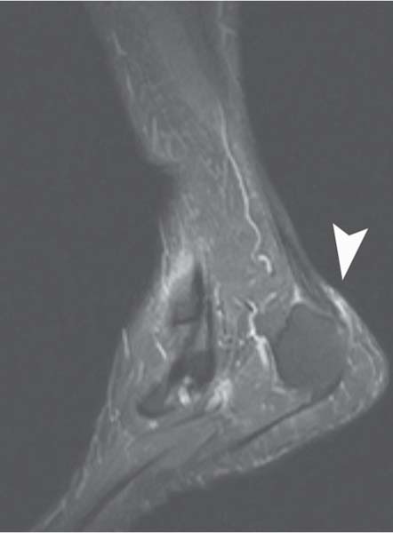
9 The Foot and Ankle

Indiscriminate use of MRI can confuse the clinical situation by identifying findings that are not necessarily pathologic or that are poorly correlated with clinical symptoms; these findings in turn can lead to unnecessary and costly interventions and can delay proper diagnosis and treatment.1 MRI of the foot and ankle has improved with the development of high-field systems and enhanced surface coil technology. Most centers use a standard screening examination, consisting of an array of specified imaging planes and pulse sequences. For the ankle, the patient is imaged in a supine, feet-first position with the malleoli several centimeters inferior to the center of the coil; images are obtained in the axial, coronal, and sagittal planes relative to the tabletop. Imaging of the foot is performed in so-called oblique planes, which are parallel and perpendicular to the long axis of the meta-tarsals, and with minimal plantarflexion to accentuate the fat plane between the peroneal tendons, improve visualization of the calcaneofibular ligament, and decrease the magic angle effect.²

In addition to standard T1-weighted and T2-weighted sequences, fat-suppressed T2-weighted and STIR sequences are extremely sensitive for detecting marrow and soft-tissue pathology by accentuating the increased signal of fluid and edema relative to the surrounding structures. A proton-density pulse sequence is occasionally used, often with fat suppression; it combines characteristics of T1-weighted and T2-weighted images. These sequences are acquired with an FSE technique that produces the desired contrast in a fraction of the time needed for conventional T2-weighted sequences, minimizing patient motion, improving throughput, and providing great benefit for claustrophobic patients. Novel developments such as parallel imaging techniques,³ combined with increased signal-to-noise ratio at higher field strengths, may continue to reduce scan times.

Imaging parameters can also be refined for optimal cartilage visualization (see Chapter 14). Gradient-echo sequences are often used to evaluate ligaments and articular cartilage (see Chapter 14), particularly in the coronal plane, allowing for optimal visualization of the articular cartilage within the mortise joint. However, early reports comparing cartilage imaging within the ankle at 3.0 T and 1.5 T have suggested that coronal intermediate-weighted FSE sequences result in better images than do fat-suppressed gradient-echo–based sequences at 3.0 T, primarily because of increased artifact at higher field strength on gradient-echo sequences.⁴ In addition, gradient-echo sequences should be avoided in the presence of indwelling metal hardware because of the technique’s inherent increased artifact (see Chapter 1).

MR arthrography can be performed as a direct or indirect method. Direct MR arthrography is performed by injecting approximately 10 mL of diluted gadolinium contrast agent into the ankle joint from an anterior approach, entering just medial to the tibialis anterior tendon with slight cranial angulation; care should be taken to avoid the course of the dorsalis pedis artery.⁵ Postinjection imaging sequences typically include fat-suppressed T1-weighted and T2-weighted images. Indirect MR arthrography is performed by injecting gadolinium intravenously and imaging the joint after contrast has been taken up by the synovium and then diffused into the joint.

Direct MR arthrography of the ankle can improve visualization of acute and chronic ligamentous injuries, particularly those involving the LCL complex, although arthrography can also be useful for visualizing syndesmotic and deltoid ligament tears. MR arthrography has also been shown to be an accurate technique for visualizing intraarticular pathology in the various ankle impingement syndromes, in differentiating stage II from stage III osteochondral talar lesions, and in identifying loose bodies and synovial disorders.⁵ Indirect MR arthrography is limited by the lack of joint distention and by inferior contrast relative to direct arthrography, although it can be a useful adjunct to MRI for the assessment of the following⁵:

• Subtle cartilage defects

• Osteochondral talar lesions

• Ligamentous injuries

• Synovitis

• Sinus tarsi syndrome

However, with the advent of high-field, high-resolution imaging and novel noncontrast MR techniques, direct and indirect MR arthrography techniques may be rendered obsolete in the future.

Traumatic Conditions

Bone contusion represents an injury to the internal bone structure with microtrabecular disruption, but no gross cortical fracture. On MRI, bone contusion appears as a focal area of low signal on T1-weighted images with ill-defined margins; high signal on T2-weighted images signifies edema within the bone marrow but an intact cortical structure6 (Fig. 9.1). Bone bruises may be seen after direct trauma or after acute ankle sprains.^6,7 Certain bone-bruise patterns are characteristic for specific injury mechanisms. For example, inversion injuries are associated with contusion of the medial malleolus and medial talus (with signal changes seen in those structures), whereas a plantarflexion mechanism can result in a posterior tibial bone bruise. Jamming injuries of the hallux may result in a bone contusion of the first metatarsal head dorsally, but direct impact on the ball of the foot may result in contusion of a sesamoid. Acute bone bruises typically resolve within 2 to 3 months unless there is ongoing repetitive injury.

Ligament Sprains

Ankle sprains are an extremely common injury, both during sports and during daily activities. The vast majority can be diagnosed with a detailed history, careful physical examination, and ankle radiographs to exclude acute fracture. MRI is not necessary for most acute ankle sprains, but it can be of use in certain cases of atypical presentation or to rule out other injuries such as an OCD or tendon injury. Within the first week after an ankle sprain, MRI usually reveals prominent subcutaneous edema and juxtaarticular hematoma; these findings present as high signal fluid in the ankle joint and adjacent tendon sheaths on T2-weighted images, indicating the presence of blood within these compartments.^6,8 The edema typically diminishes rapidly thereafter, although fascial edema around the injured ligament may persist.^6,8 After the first several weeks, the ligament becomes thickened and may appear in continuity despite a tear, which may confound accurate interpretation. Two months after injury, fascial edema is resolved and the torn ligaments may appear intact, thinned, attenuated, or even completely absent, depending on the degree of initial injury.^6,8

Ankle sprains are the most common athletic injury, and specifically, lateral ankle ligament sprains are the most common type.9 Ankle sprains account for 45% of basketball injuries,¹⁰ and are commonly seen in football, soccer, rugby, and volleyball players. These injuries vary in severity from mild to severe^6,10; lateral ligament injuries are more common than medial ones.^9,10 The most commonly injured ligament is the anterior talofibular ligament, followed by a combination injury of the calcaneofibular and anterior talofibular ligaments. An isolated posterior talofibular ligament tear is rare. The most common mechanism of injury is inversion and internal rotation. It must be noted that this mechanism can also produce other common injuries, in isolation or in combination with ankle sprain, such as the following:

• Fibular or talar fractures

• Osteochondral lesions

• Peroneal tendon tears

• Fifth metatarsal fractures

The diagnosis of ankle sprain is usually accomplished with a thorough history and physical examination. Conventional radiographs may reveal any associated avulsion fractures or osteochondral injuries, and stress views can be obtained to evaluate structural instability. Occasionally, MRI is used to confirm the diagnosis or for the evaluation of associated injuries. Ligament injuries are best evaluated on T2-weighted and fat-suppressed T2-weighted MR images. These images usually show increased signal intensity that represents the edema and fluid collection secondary to trauma.^6,8 Discontinuity of the ligament on T1-weighted and T2-weighted images signifies disruption.^6,8 The anterior talofibular ligament is the weakest and the most vulnerable of all ankle ligaments. Tears in this ligament are best diagnosed on axial images (Fig. 9.2).

The second most common pattern of ankle injury is a combined injury to the anterior talofibular ligament and the calcaneofibular ligament.10 Isolated tears of the calcaneofibular ligament are extremely uncommon.¹⁰ Unlike the anterior talofibular ligament, tears of the calcaneofibular ligament are best seen on the coronal T2-weighted, fat-suppressed T2-weighted, and fat-suppressed STIR images (Fig. 9.3). MRI grading of the ligamentous injury can be categorized as follows⁶:

Isolated injuries of the deltoid ligament are uncommon.10 They often occur in conjunction with a fibular fracture or a purely ligamentous syndesmotic injury. Deltoid ligament injuries are best viewed on coronal T2-weighted and fat-suppressed T2-weighted images (Fig. 9.4). Occasionally, medial edema and deltoid thickening are seen on T2-weighted images secondary to an inversion injury.⁶ This medial impaction is usually associated with lateral soft-tissue edema or evidence of a lateral ligament tear. MR images must be correlated carefully with clinical examination to avoid treatment of false-positive findings.

Syndesmotic Injuries11,12

Also sometimes called high ankle sprains, syndesmotic sprains are reported to occur in as many as 18% of all ankle sprains in athletes.¹³ Syndesmotic injury usually is associated with a fibular fracture, but it can occur as a purely ligamentous diastasis.^12,14 The major contributors to the distal tibiofibular syndesmotic structure are the following:

• Anteroinferior tibiofibular ligament

• Posteroinferior tibiofibular ligament

• Interosseous membrane

The anteroinferior tibiofibular ligament is most commonly involved in syndesmotic injuries. External rotation is the typical mechanism of injury, and many of these injuries are not recognized initially unless the clinician has a high level of suspicion for them.¹³ Patients typically present with severe edema, ecchymosis, and tenderness more laterally than would be expected with a standard lateral ligament sprain. Clinical examination is supplemented with radiographic studies to exclude fibular fracture or diastasis of the syndesmosis. One study has indicated that the measurements on static ankle radiographs are poorly predictive of syndesmotic injury.¹¹ Dynamic stress radiographs may identify instability of the syndesmosis, but they may be limited in the acute setting because of patient discomfort.

MRI has been found to very useful in identifying these injuries. In one study, MRI had a sensitivity of 100%, a specificity of 93%, and an accuracy of 97% in diagnosing syndesmotic injuries.¹² The anteroinferior tibiofibular ligament and posteroinferior tibiofibular ligament are best viewed in axial images at the level of the tibial plafond. When injured, the ligaments can be seen as edematous, wavy, absent, or discontinuous on T1-weighted and T2-weighted sequences (Fig. 9.5A). Extension of fluid into the syndesmosis on axial T2-weighted images can also assist in the diagnosis of syndesmotic disruption (Fig. 9.5B).

OCD of the Talus

OCD, also known as an osteochondral fragment of the talus, is a disruption of that structure’s cartilage surface. Analogous lesions are common in the knee and elbow. Many occur after a traumatic injury, although some patients do not recall a specific injury. An OCD lesion often is misdiagnosed clinically as an ankle sprain.^15,16 Patients typically present with pain located deep within the joint that is worsened with activity or sports; patients may also complain of ankle swelling, giving way, or locking.

OCD lesions can occur anywhere on the surface of the talar dome; the classic literature notes anterolateral and posteromedial lesions as the most common.15,17 A recent MRI study identified the centromedial and centrolateral locations as the most common.¹⁸

A spectrum of OCD lesions exists, including the following^16,19:

• Softening of the cartilage

• Partial detachment of an osteochondral fragment

• Complete detachment of an osteochondral fragment

• Free-floating fragment within the joint

• Subchondral cystic lesion

Stable lesions may respond to nonsurgical treatment, whereas unstable lesions and cystic OCD lesions typically are treated surgically.

MRI is a very useful modality for diagnosing OCD lesions, particularly if the lesion is not visualized on standard radiographs. MRI can also assess other pathologic entities, such as tendon or ligamentous injuries, in the patient with persistent pain after ankle sprain. All three imaging planes can be useful in assessing OCD lesions. The AP location can be determined on axial and sagittal images, whereas the mediolateral location can be assessed on coronal and axial views. The depth of the lesion can be viewed on sagittal and coronal images. The MRI appearance of an OCD lesion typically shows osseous edema along with irregularity of the subchondral bone plate and overlying cartilage (Fig. 9.6). Specialized cartilage-specific sequences can improve imaging of the chondral surface to identify subtle disruption²⁰ (see the detailed discussion in Chapter 14). In some cases, the surrounding bone edema may cause overestimation of the true size of the lesion. MRI appearance also may assist in predicting the stability of the lesion; fluid or granulation tissue beneath the lesion at the interface with the osseous crater appears bright on T2-weighted imaging and implies instability^21–23 (Fig. 9.7). MRI has also been shown to be of use in evaluating healing of the OCD lesion after surgery, with some normalization of signal changes noted.^24,25

Stress Fractures

Osseous stress fractures occur from repetitive stress that is below the threshold for acute fracture but substantial enough to cause microtrabecular failure. They often occur secondary to overuse situations, such as in an athlete with a sudden, dramatic increase in running or other training. The bone is unable to heal adequately because of ongoing insult, and a stress fracture results. These fractures are typically diagnosed based on a history of repetitive overuse and are differentiated from acute fractures by the lack of an acute traumatic event. The location of lower extremity stress fractures in a group of military recruits has been reported to vary by gender: the most common sites in males were the metatarsals (66%), calcaneus (20%), and lower leg (13%), whereas the most common sites in females were the calcaneus (39%), metatarsals (31%), and lower leg (27%).²⁶ Furthermore, conventional radiographs usually are negative early in the process until callus appears or the stress fracture progresses to a frank fracture. One study found a rate of positive radiographic findings of only 10% in patients with stress fractures.²⁷ MRI is a very helpful tool in evaluating these injuries, with high sensitivity and specificity. Typically, the osseous structures have a linear region of low signal intensity on T1-weighted and T2-weighted images; T2-weighted images also show surrounding high signal intensity consistent with bone marrow edema.⁶

Calcaneal Stress Fractures

A patient with a calcaneal stress fracture presents with posterior heel pain and, occasionally, swelling. On physical examination, pain is elicited with medial-lateral compression of the heel. Sometimes conventional radiographs can show a radiolucent line at the posterior aspect of the calcaneus perpendicular to the trabecular cancellous lines. MRI is useful if radiographs are negative, with T1-weighted images showing a linear fracture line and T2-weighted images revealing associated marrow edema (Fig. 9.8).

Navicular Stress Fractures

Navicular stress fractures commonly present in an athlete who complains of vague arch pain that is worsened with running or sports activities. The stress fracture usually occurs in the middle third of the navicular secondary to increased stresses in that region along with poor local vascular supply to the bone. MRI typically shows edema within the navicular on T2-weighted and fat-suppressed T2-weighted images (Fig. 9.9A). T1-weighted images show a low intensity linear lesion representing a fracture line (Fig. 9.9B). If MRI suggests a navicular stress fracture, a CT scan may be indicated to define more clearly the osseous structure and extent of the fracture.

Metatarsal Stress Fractures

Metatarsal stress fractures are also called march fractures because they often present in military recruits who participate in extended marching drills. Metatarsal stress fractures also commonly present in female dancers who are often in the en-pointe position and in female athletes, both of whom subject the central metatarsals to increased mechanical load. The second metatarsal is the most frequent location for fracture (more than half of all metatarsal stress fractures), followed by the third and fourth metatarsals.²⁸ Stress fractures of the central metatarsals typically occur in the diaphysis, whereas a stress fracture of the first metatarsal occurs in the proximal metaphysis and a stress fracture of the fifth metatarsal occurs at the diaphyseal-metaphyseal junction.²⁸ Patients typically complain of aching pain related to weight-bearing activities, running, or sports. Conventional radiographs often are diagnostic, although they may be negative early in the process. MRI can be useful in such cases and to rule out other causes of pain such as synovitis. The metatarsal shows the characteristic linear density on T1-weighted images with high signal on corresponding T2-weighted and fat-suppressed T2-weighted images (Fig. 9.10).

Tendon disorders can represent traumatic injuries, inflammatory conditions, or degenerative tendinosis. Regardless of the etiology, MRI is the ideal method of evaluating tendon disorders and is best achieved by obtaining images perpendicular to the tendon’s course.29–33 At the ankle and hindfoot levels, axial views are ideal for tendon imaging, whereas coronal images are best for visualizing more distal structures in the midfoot. The magic angle effect is a phenomenon seen in tissues with well-ordered collagen fibers, such as a tendon.³⁴ This phenomenon occurs when the images are obtained with the magnetic field at an oblique angle (55 degrees) relative to the fibers of the tendon, and it shows abnormal signal intensity on T1-weighted images. T2-weighted images are unaffected by this phenomenon, so corresponding T2-weighted images are scrutinized in the affected areas to determine if the signal abnormality seen on T1-weighted images represents true pathology or simply artifact. The magic angle effect is seen most notably in the posterior tibialis and peroneal tendons as they course around the malleoli. Knowledge that this magic angle effect exists, combined with assessment of the T2-weighted images, assists the radiologist or surgeon in accurately identifying pathology of the tendons about the ankle.

Isolated retrocalcaneal bursitis can be seen secondary to systemic inflammatory disease or localized soft-tissue irritation from impingement by the posterosuperior process of the calcaneus (Haglund process). Sagittal MR images show decreased signal intensity on T1-weighted images and increased intensity on T2-weighted and fat-suppressed T2-weighted images, consistent with soft-tissue inflammation6 (Fig. 9.11

Related posts:

MRI Safety Essentials of MRI Physics and Pulse Sequences Advanced Techniques in Musculoskeletal MRI The Shoulder A Systematic Approach to the Review of Musculoskeletal MRI Studies The Cervical Spine

Stay updated, free articles. Join our Telegram channel

Join